Table of Contents
This set of tutorials covers the basics of the Tridash programming language.
Prior programming experience is not strictly necessary however is helpful.
The full source code for these tutorials is available in the tutorials directory of the Tridash source: https://github.com/alex-gutev/tridash/tree/master/tutorials. |
A Tridash program is made up of a number of components called nodes, which are loosely analogous to variables in other languages. Each node holds a particular value, referred to as the node’s state, at a given moment in time.
Nodes are created the first time they are referenced, by their
identifiers. Node identifiers can consist of any sequence of
Unicode characters excluding whitespace, parenthesis (, ), braces
{, }, double quotes " and the following special characters: ;,
,, ., #. A node identifier must consist of at least one
non-digit character otherwise it is interpreted as a number.
The following are examples of valid node identifiers:
-
name -
full-name -
node1 -
1node
There are few restrictions on the characters allowed in node
identifiers, meaning node identifiers may even contain symbols such as
|
A node can be bound to another node in which case its value is automatically updated when the value of the node, to which it is bound, changes.
The -> operator establishes a binding between the node on the left
hand side, referred to as the source, and the node on the right hand
side, referred to as the target.
Example.
a -> b
The spaces between the node identifiers and the bind |
In this example a binding is established between node a and node
b. The result is that when the value of a changes, the value of
b is automatically updated to match the value of a. This kind of
binding is known as a simple binding since a node is simply set to the
value of another node. Node a is referred to as a dependency node
of b, since b's value depends on the value of a, and b is
referred to as an observer node of a since it actively observes
its value.
We’ll use bindings to develop a simple application which asks for the user’s name and displays a greeting.
This tutorial targets the JavaScript backend and makes use of HTML for the user interface.
Some knowledge of the basics of HTML, i.e. what tags, elements and attributes are, is necessary to complete this tutorial. |
We’ll start off by creating an HTML file, called hello-ui.html, with
the following contents:
hello-ui.html.
<?
 self.input-name.value -> name
 name -> self.span-name.textContent
?>

<!doctype html>
<html>
    <head>
        <title>Hello Node</title>
    </head>
    <body>
        <h1>Tutorial 1: Hello Node</h1>
        <label>Enter your name: <input id="input-name"/></label>
        <p>Hello <span id="span-name"></span></p>
    </body>
</html>
Most of the file is HTML boilerplate, the interesting part is within
the <? ... ?> tag. The content of this tag is interpreted as Tridash
code. Tridash code tags can be placed almost anywhere in the file,
we’ve just chosen to place it at the top.
The Tridash code consists of two explicit binding
declarations. Declarations are separated by a line break or a
semicolon ;.
Tridash Code.
self.input-name.value -> name
name -> self.span-name.textContent
The declaration in the first line binds the self.input-name.value
node to the name node.
The node self.input-name is a special node that references the
input element, with id input-name, in the HTML file. HTML elements
can be referenced from within Tridash code, in the same HTML file,
using the expression self.<id> where <id> is substituted with the
id of the element.
The |
The node self.input-name.value, which references the value
attribute of the HTML element with ID input-name, is bound to the
node name. Thus whenever the value of input-name.value changes,
the value of name is set to it. In other words, whenever text is
entered in the input element, the value of name is automatically set
to the text entered.
In the second declaration, the name node is bound to the
self.span-name.textContent node. self.span-name references the
HTML span element with ID span-name, with the node
self.span-name.textContent referencing the textContent attribute,
i.e. the content, of the element. The result of this binding is that
whenever the value of the name node changes, its value is displayed
in the span element. As mentioned earlier, the value of the name
node is automatically set to the text entered in the input element,
thus the value entered in the input element is displayed in the
span element.
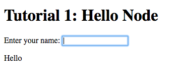
The application we’ve just written, simply prompts the user for his/her name and displays “Hello” followed by the user’s name directly below the prompt. Let’s try it out to see if it works.
Run the following command to build the application:
tridashc hello-ui.html : node-name=ui -o hello.html -p type=html -p main-ui=ui
That looks complicated, let’s simplify it a bit.
The tridashc executable compiles one or more Tridash source files,
generating an output file. The source files, in this case
hello.html, are listed after tridashc. The name of the output file
is given by the -o or --output-file option, in this case
hello.html.
The snippet : node-name=ui sets the node-name option, for
processing the source file hello-ui.html, to ui. This creates a
node ui with which the contents of the HTML file can be referenced.
The |
The -p option=value command-line options sets various options
related to the compilation output. The first option type is set to
html which indicates that the output should be an HTML file with the
generated JavaScript code embedded in it. The main-ui option is set
to ui, which is the name of the node referencing the contents of the
hello-ui.html file. It is the contents of this file that are used to
generate the output HTML file.
If all went well a hello.html file should have been created in the
same directory, after running the command.
Open the hello.html file in a web-browser with JavaScript
enabled. You should see something similar to the following:
Try entering some text in the text field, and press enter afterwards:
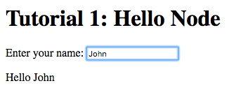
Notice that the text entered appears next to the “Hello” message
underneath the text field. This is due to the binding of the text
field to the name node and the binding of the name node to the
contents of the span element placed adjacent to the “Hello” text.
Now try changing the text entered in the text field:
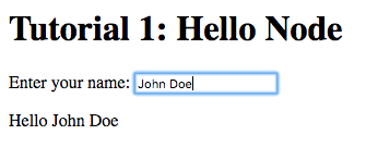
The text changes to match the contents of the text field. This demonstrates the automatic updating of a node’s state when the state of its dependency nodes changes.
When the state (the value) of the text field changes:
-
The state of the
namenode is updated to the text entered in the field. -
The content of the
spanelement is updated to match the state of thenamenode.
The previous application can be implemented much more succinctly using implicit bindings and inline node declarations.
hello-ui.html.
<!doctype html>
<html>
    <head>
        <title>Hello Node</title>
    </head>
    <body>
        <h1>Tutorial 1: Hello Node</h1>
        <label>Enter your name: <input value="<?@ name ?>"/></label>
        <p>Hello <?@ name @></p>
    </body>
</html>
Implicit bindings between an HTML node and a Tridash node can be
established using the <?@ declaration ?> tag. This is similar to the
Tridash code tag, seen earlier, however an implicit binding is
established between the nodes appearing in the tag and the HTML node
in which the tag appears.
If the tag is placed within an attribute of an element, an implicit
two-way binding is established between the element’s attribute and the
node, appearing in the tag. If the tag appears outside an attribute,
an HTML element is created in its place, and a binding is established
between the node appearing in the tag, and the content of the element
(referenced as textContent from Tridash).
With inline declarations it is not necessary to give the HTML elements unique ID’s unless they will be referenced from within Tridash code. In this example they have been omitted.
The bindings we’ve seen so far are one-way bindings, as data only flows in one direction, from the dependency node to the observer node.
Example: One-Way Binding.
a -> b
This is a one-way binding since the value of b is updated to the
value of a when it changes, however, a is not updated when the
value of b changes.
If a binding in the reverse direction is also established:
b -> a
the binding becomes a two-way binding since the value of each node is updated when the value of the other node changes.
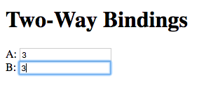
The following simple application demonstrates two-way bindings:
ui.html.
<?
 a -> b
 b -> a
?>

<!doctype html>
<html>
  <head>
    <title>Two-Way Bindings</title>
  </head>
  <body>
    <h1>Two-Way Bindings</h1>
    <div><label>A: <input value="<?@ a ?>"/></label></div>
    <div><label>B: <input value="<?@ b ?>"/></label></div>
  </body>
</html>
The applications consists of two text input fields with the first
field bound to node a and the second field bound to b, using
inline node declarations.
In the Tridash code tag, a two-way binding between a and b is
established since a binding is declared in both directions:
-
a -> b -
b -> a
Build the application using the following command, which is identical to the previous build command with only the source and output file names changed.
tridashc ui.html : node-name=ui -o app.html -p type=html -p main-ui=ui
Open the resulting app.html file in a web-browser, and enter a value
in the first text field:
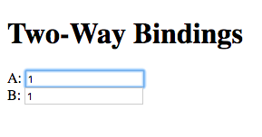
Notice that the content of the second text field is automatically updated to match the content of the first field.
Now change the value in the second field:
The value of the first field is updated to the value entered in the second field.
The bindings in the previous tutorial were pretty boring and limited. Whatever was entered in the text field was simply displayed below it, verbatim. In-fact, this functionality is already offered by many web frameworks and GUI toolkits. The real power of the Tridash language comes from the ability to specify arbitrary functions in bindings which are dependent on the values of more than a single node. Moreover these bindings can be established in Tridash itself without having to implement "transformer" or "converter" interfaces/subclasses in a lower-level language.
A functor node is a node which is bound to a function of the values of one or more nodes. It consists of an expression comprising an operator applied to one or more arguments.
Functor Node Syntax.
operator(argument1, argument2, ...)
A binding is established between the argument nodes and the functor node. Whenever the value of one of the argument nodes changes, the expression is reevaluated and the value of the functor node is updated.
Example: Functor of one argument.
to-int(a)
The functor node is to-int(a) consisting of the function to-int,
which converts its argument to an integer, applied to the value of
node a. When the value of a changes, the value of to-int(a) is
updated to a's value converted to an integer.
Example: Functor of two arguments.
a + b
This is a functor node of the function + which computes, you guessed
it, the sum of its arguments, in this case a and b. Whenever the value
of either a or b changes, the value of a + b is updated to the
sum of a and b.
The |
The spaces between an infix operator and its arguments are
mandatory since |
Functor nodes can be bound to other nodes using the same -> operator.
Example: Binding functors to other nodes.
a + b -> sum
In this example node sum is bound to a + b which is bound to the
sum of a and b.
We’ll build an application which computes the sum of two numbers, entered by the user, and displays the result.
Let’s focus on building the interface for now. Begin with the
following ui.html file:
ui.html.
<!doctype html>
<html>
    <head>
        <title>Adding Numbers</title>
    </head>
    <body>
      <h1>Adding Numbers</h1>
      <div><label>A: <input value="<?@ a ?>"/></label></div>
      <div><label>B: <input value="<?@ b ?>"/></label></div>
      <hr/>
      <div><strong>A + B = <?@ sum ?></strong></div>
    </body>
</html>
An interface consisting of two text input fields is created. The first
field is bound to node a and the second to node b. Underneath the
fields the node sum is bound to an unnamed HTML element located next
to “A + B =”.
Nodes a and b are bound to the values of the two numbers. Node
sum is to be bound to the sum of a and b.
Before we begin writing the binding declarations we need to import the
nodes from the core module, you’ll learn more about modules in a
later tutorial, which we’ll be making use of in this application. The
following imports all nodes from the core module:
Import all nodes from module core.
/import(core)
Nodes a and b are bound to the contents of the text fields,
however the contents of the text fields are strings. We need to
convert a and b to integers in order to compute the sum. This is
achieved using the to-int operator.
The sum of the integer values of a and b is computed using the +
operator applied on the arguments to-int(a) and
to-int(b).
Computing Sum of a and b.
to-int(a) + to-int(b)
Finally, we need to bind the sum to the node sum in order for it to
be displayed below the fields.
to-int(a) + to-int(b) -> sum
Adding the declarations, we’ve written so far, to a Tridash code tag (somewhere in the file such as at the beginning), completes the application.
Tridash Code Tag.
<?
 /import(core)

 to-int(a) + to-int(b) -> sum
?>
To simplify the build command, the build options are specified in a build configuration file.
The build configuration file contains the list of sources, along with the source-specific options, and the output options in YAML syntax (see https://yaml.org for details).
Create the following build.yml file:
build.yml.
sources:
  - path: ui.html
    node-name: ui

output:
  path: app.html
  type: html
  main-ui: ui
The outer structure of the file is a dictionary with two entries
sources and output.
The sources entry contains the list of source files either as a path
or as a dictionary with the path in the path entry and the
processing options in the remaining entries. In this application there
is one source file ui.html with one source processing option
node-name set to ui.
The output entry is a dictionary containing the path to the output
file in the path entry, in this case app.html, and the output
options in the remaining entries, in this case type = html and
main-ui = ui which are the same options as in the previous
tutorials.
To build from a build configuration file run the following command:
tridashc -b build.yml
The -b option specifies the path to the build configuration file
containing the build options. All other command line options are
ignored when this option is specified.
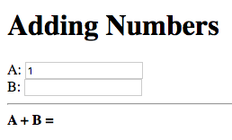
Open the app.html file in a web browser, and enter some
numbers in the text fields:
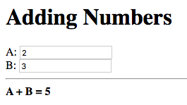
Notice that the sum of the numbers is automatically computed and displayed below the fields.
The sum will only be displayed once you have entered a valid number in each field. |
Now try changing the numbers (remember to press enter afterwards):
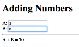
Notice that the sum is automatically recomputed and the new sum is displayed.
The to-int operator is special in that a two-way binding is
established between its argument and the functor node. Thus the
declaration to-int(a) also establishes the binding to-int(a) -> a.
The binding in the reverse direction, from functor to argument, has
the same function as the binding from the argument to the
functor. Thus in to-int(a) -> a, a is bound to the value of
to-int(a) converted to an integer.
This allows a binding to be established with a to-int functor node
as the observer.
Example: Binding with to-int as observer.
x -> to-int(a)
In this example, to-int(a) is bound to x. Whenever the value of
x changes, the value of to-int(a) is set to it, and the value of
a is set to the value of to-int(a) converted to an integer.
With this functionality, the application in this tutorial can be implemented more succinctly by moving the integer conversion from the Tridash code tag to the inline node declarations.
Replace the declaration:
to-int(a) + to-int(b) -> sum
with:
a + b -> sum
Replace <?@ a ?> and <?@ b ?> with <?@ to-int(a) ?> and <?@
to-int(b) ?> respectively.
The benefit of this is that the value conversion logic is moved closer
to the point where the values are obtained, rather than being littered
throughout the core application logic. Nodes a and b can now be
used directly, without having to be converted first, since it is known
that they contain integer values.
To simplify the application further, the sum node can be omitted
entirely and <?@ sum ?> can be replaced with <?@ a + b ?>.
Improved Application.
<?
 /import(core)
?>
<!doctype html>
<html>
    <head>
        <title>Adding Numbers</title>
    </head>
    <body>
      <h1>Adding Numbers</h1>
      <div><label>A: <input value="<?@ to-int(a) ?>"/></label></div>
      <div><label>B: <input value="<?@ to-int(b) ?>"/></label></div>
      <hr/>
      <div><strong>A + B = <?@ a + b ?></strong></div>
    </body>
</html>
The |
This tutorial introduces functionality for conditionally selecting the value of a node.
The special case operator selects the value of the first node for
which the value of the corresponding condition node is true. The
case operator is special in that it has a special syntax to make it
more readable.
The |
Syntax.
case(
  condition-1 : value-1,
  condition-2 : value-2,
  ....
  default-value
)
Each argument is of the form condition : value where condition is
the condition node and value is the corresponding value node. The
last argument may also be of the form value, that is there is no
condition node, in which case it becomes the default or else value.
The case functor node evaluates to the value of the value node
corresponding to the first condition node which has a true value
(equal to the value of the builtin node True), or the value of the
default node, if any, when all condition nodes have a false (equal
to the value of the builtin node False) value.
Example.
case(
  a > b : a - b
  b > a : b - a
  0
)
If the node a > b evaluates to true, the case node evaluates to
the value of a - b, otherwise if b > a evaluates to true, the
case node evaluates to the value of b - a. If neither a > b nor
b > a evaluate to true, the case node evaluates to 0.
If the default value node is omitted and no condition node evaluates
to true, the case node evaluates to a failure value (you will learn
about failure values in a later tutorial which introduces error
handling).
Let’s write a simple case expression which returns the maximum of
two numbers, a and b, and returns the string “neither” when
neither number is greater than the other.
The case expression should evaluate to:
-
aifa > b -
bifb > a - The string “neither” otherwise
These conditions are implemented by the following case expression:
case(
    a > b : a,
    b > a : b,
    "neither"
)
)
| This is the literal string “neither”. |
String constants are written in double quotes |
Notice that the last argument does not have an associated
condition. The case node evaluates to this argument if none of the
conditions, of the previous arguments, evaluate to true.
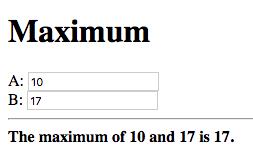
We can incorporate this in a simple application, which displays the maximum of two numbers entered by the user, using the following HTML interface:
ui.html.
<?
 /import(core)

 maximum <-
     case (
         a > b : a,
         b > a : b,
         "neither"
     )
?>
<!doctype html>
<html>
    <head>
        <title>Maximum</title>
    </head>
    <body>
      <h1>Maximum</h1>
      <div><label>A: <input value="<?@ to-int(a) ?>"/></label></div>
      <div><label>B: <input value="<?@ to-int(b) ?>"/></label></div>
      <hr/>
      <div><strong>The maximum of <?@ a ?> and <?@ b ?> is <?@ maximum ?>.</strong></div>
    </body>
</html>
The |
The interface consists of two text fields, the contents of which are
bound to nodes a and b. The to-int operator is used to convert
the string values to integers as in the previous tutorial.
The node maximum is bound to the value of the case functor, and
its value is displayed in an unnamed HTML element below the input
fields.
The values of |
Build and run the application, using the same build configuration file and command from the previous tutorials.
Enter some numbers in the text fields:
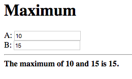
Notice that the maximum, 15 in this case, is displayed below the text fields. Also notice that the values entered in the text fields are displayed as part of the message.
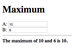
Now change the number, which is the maximum, to a different value which is still greater than the other number:
The new maximum is displayed. This demonstrates that if the values of
the value nodes, of the case expression change, the value of the
case expression is updated.
Change the maximum number such that it is smaller than the other number:
This shows that the value of the case expression is also updated if
the values of the condition nodes change.
Now finally change the numbers such that they are both equal:
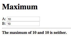
The displayed maximum is “neither” which is the default value of the case expression.
Let’s extend the application developed during the previous tutorial by adding the functionality for specifying a limit to the sum of the two numbers. The application should inform the user of whether the limit was exceeded.
Start with the following slightly modified code from the previous tutorial.
<?
 /import(core)

 a + b -> sum
?>
<!doctype html>
<html>
    <head>
        <title>Sum Limit</title>
    </head>
    <body>
      <h1>Sum Limit</h1>
      <div><label>Limit: <input value="<?@ to-int(limit) ?>"/></label></div>
      <hr/>
      <div><label>A: <input value="<?@ to-int(a) ?>"/></label></div>
      <div><label>B: <input value="<?@ to-int(b) ?>"/></label></div>
      <hr/>
      <div><strong>A + B = <?@ sum ?></strong></div>
    </body>
</html>
A new text input field for the limit has been added, with its value
bound to the node limit.
The sum |
The message “Within limit.” should be displayed if the sum is less
than the limit (sum < limit), and “Limit Exceeded!”
otherwise. This can be implemented using the following case
expression, which is bound directly to an unnamed element.
Add the following below the element where the sum is displayed.
<div>
  <?@
    case(
        sum < limit : "Within Limit.",
        "Limit Exceeded!"
    )
  ?>
</div>
There is no difference in efficiency between using the |
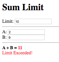
Build and run the application, and enter some initial values for the
limit, a and b.
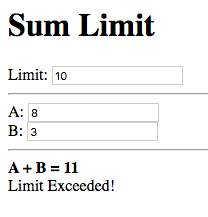
“Limit Exceeded!” is displayed since the sum of 11 did indeed exceed the limit of 10, with the numbers in the snapshot above.
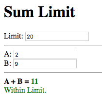
Now try increasing the limit:
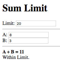
The message changes to “Within Limit.”.
Whilst the application we’ve implemented so far demonstrates the power of functional bindings, it is rather lacking in that whether the limit has been exceeded or not is only indicated by text. The text has to be read in full to determine whether the limit was exceeded, and changes from Within Limit to Limit Exceeded, and vice versa, are hard to notice. Some visual indications, such as a change in the color of the sum, when the limit is exceeded, would be helpful.
As an improvement, we would like the text color of the the sum, and the status message, to be red when the sum exceeds the limit, and to be green when it is within the limit.
Let’s start off by giving an ID to the elements in which the sum and
status message are displayed, so that they can be referenced from
Tridash code. Surround <?@ sum ?> in a span element with ID sum
and assign the div element, containing the status message, the ID
status.
<div><strong>A + B = <span id="sum"><?@ sum ?></span></strong></div>
<div id="status">
  <?@
    case(
        sum < limit : "Within Limit.",
        "Limit Exceeded!"
    )
  ?>
</div>
Let’s create a node color which will be bound to the text color in
which the sum and status message should be displayed. It should have
the value "green" when the sum is within the limit and the value
"red" when the sum exceeds the limit. This can be achieved by
binding to a case functor node.
The values |
Add the following to the Tridash code tag.
case(
  sum < limit : "green",
  "red"
) -> color
The value of the case functor node is "green" if sum is less
than limit and "red" otherwise. The case functor node is bound to
the color node.
The color node somehow has to be bound to the text color of the
sum and status elements. Text color is a style attribute of an
element. All style attributes are grouped under a single subnode
style of the HTML element node. The text color is controlled by the
color attribute, referenced using style.color.
The color node is bound to the style attributes of the elements with
the following (add to the Tridash code tag):
color -> self.sum.style.color
color -> self.status.style.color
Full ui.html code:
ui.html.
<?
 /import(core)

 a + b -> sum

 case (
     sum < limit : "green",
     "red"
 ) -> color

 color -> self.sum.style.color
 color -> self.status.style.color
?>
<!doctype html>
<html>
    <head>
        <title>Sum Limit</title>
    </head>
    <body>
      <h1>Sum Limit</h1>
      <div><label>Limit: <input value="<?@ to-int(limit) ?>"/></label></div>
      <hr/>
      <div><label>A: <input value="<?@ to-int(a) ?>"/></label></div>
      <div><label>B: <input value="<?@ to-int(b) ?>"/></label></div>
      <hr/>
      <div><strong>A + B = <span id="sum"><?@ sum ?></span></strong></div>
      <div id="status">
        <?@
          case(
              sum < limit : "Within Limit.",
              "Limit Exceeded!"
          )
        ?>
      </div>
    </body>
</html>
Build and run the application. Enter some values for a, b and the
limit such that the sum exceeds the limit.
The status message and sum are now shown in red which provides an immediate visual indication that the limit has been exceeded.
Now increase the limit, or decrease the values of a and b:
The color of the status message and sum is immediately changed to green, which provides a noticeable indication that the limit has no longer been exceeded.
In this tutorial you’ll learn how to create your own functions, which can be used in functional bindings. Another feature which distinguishes Tridash from frameworks/toolkits, which offer bindings, is that new functions can be written in the same language, as the language in which the bindings are declared, rather than having to be implemented in a lower-level language.
Only some of the example applications will be demonstrated. Visit the source code for the tutorials to try out the remaining applications. |
New functions, referred to as meta-nodes, are defined using the
special : operator, which has the following syntax:
function(arg1, arg2, ...) : {
   declarations...
}
The left-hand side contains the function name (function) followed by
the argument list in brackets, where each item (arg1, arg2, …)
is the name of the local node to which the argument at that position
is bound.
The right-hand side, of the : operator, contains the declarations
making up the body of the function, which may consist of any Tridash
node declaration. The value of the last node in the declarations
list is returned by the function.
The meta-node can then be used as the operator of functor nodes, which are referred to as instances of the meta-node, declared after its definition.
The curly braces |
Example Adding Two Numbers.
# Add two numbers
|
This is a comment. Comments begin with a |
In this example, an add meta-node is defined which takes two
arguments, x and y, and returns their sum.
Our sum application can thus be rewritten as follows:
<?
 /import(core)

 # Add two numbers

 add(x, y) : x + y
?>

...

<div><label>A: <input value="<?@ to-int(a) ?>"/></label></div>
<div><label>B: <input value="<?@ to-int(b) ?>"/></label></div>

A + B is <?@ add(a, b) ?>
...
When an explicit binding to the self node is established inside a
meta-node, the value of the self node is returned rather than the
value of the last node in the meta-node’s body.
The following is an alternative implementation of the add meta-node.
add(x, y) : {
    x + y -> self
}
This is particularly useful when binding to subnodes of the self
node, which you’ll learn about later.
Meta-node arguments can be designated as optional by giving the
argument a default value. An optional argument is of the form arg :
value, where arg is the argument node identifier and value is the
default value, to which it is bound, if it is not provided.
Example.
increment(n, delta : 1) : n + delta
In this example, the argument delta is optional and is given the
default value 1 if it is not provided.
Examples.
increment(n)    # delta defaults to 1
increment(n, 2) # delta = 2
Default values don’t have to be constants, in-fact any node expression can be used as a default value. In the case that the default value is a node, then that node will be implicitly bound to all instances of the meta-node, for which the argument is not provided.
Example: Node Default Values.
# Increment `n` by `d`

increment(n, d : delta) : n + d
In this example the default value for the delta d is the value of
the global node delta. A binding between delta and each instance
of increment, for which a value for d is not provided, will be
established.
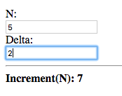
The effect of this is demonstrated in the following example application:
ui.html.
<?
 /import(core)

 # Increment `n` by `d`

 increment(n, d : delta) : n + d
?>
<!doctype html>
<html>
    <head>
        <title>Optional Argument Default Value</title>
    </head>
    <body>
      <h1>Optional Argument Default Value</h1>
      <div><label>N: <br/><input value="<?@ to-int(n) ?>"/></label></div>
      <div><label>Delta: <br/><input value="<?@ to-int(delta) ?>"/></label></div>
      <hr/>
      <div><strong>Increment(N): <?@ increment(n) ?></strong></div>
    </body>
</html>
Enter an initial value for N and Delta:
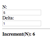
The value given to the delta (d) argument of increment is the
initial value given for Delta, which is 1.
Now try changing Delta:
The value of the increment(n) node is updated, with the new value of
Delta given as the delta argument. This shows that a binding is
established rather than simply taking the value of the delta node.
A recursive meta-node contains an instance of itself in its definition.
The following are the classic examples of recursion:
Example: Factorial.
factorial(n) :
    case(
        n < 1 : 1,  # Ignoring the case: n < 0
        n * factorial(n - 1)
    )
Example: Fibonacci Numbers.
fib(n) :
    case(
        n <= 1 : 1,
        fib(n - 1) + fib(n - 2)
    )
Recursion is the means by which Tridash provides iteration. The
definition of factorial, above, will result in the stack space being
exhausted for large values of n. This is due to the fact that each
invocation of the meta-node consumes a certain amount of stack
space. Since the recursive call to factorial has to be evaluated
before the return value of the current call can be computed, the
meta-node consumes an amount of stack space proportional to the value
of n.
If the definition is rewritten such that it is tail recursive, that is
the return value of factorial is the return value of the recursive
call, a constant amount of stack space is consumed.
Example: Tail-Recursive Factorial.
factorial(n, acc : 1) :
    case(
        n < 1 : acc,  # Ignoring the case: n < 0
        factorial(n - 1, n * acc)
    )
This definition of factorial is tail recursive since the recursive
call appears directly as the default value of the case expression,
which is simply returned without any further operations performed on
it.
In the previous implementation, the multiplication was performed on
the result of the recursive call to factorial. In this
implementation, the multiplication is performed on an accumulator
argument, acc which is passed on to the recursive call and
eventually returned when factorial is called with n < 1.
Tridash supports general tail call optimization for mutually recursive meta-nodes. |
A meta-node may contain other meta-nodes inside its definition. These meta-nodes may only be used within the body of the meta-node and shadow meta-nodes, declared in the enclosing scope, with the same identifiers.
With nested meta-nodes we can rewrite our previous tail-recursive
factorial meta-node without having to expose the accumulator
argument acc, which is an implementation detail.
Example: Factorial with nested iter meta-node.
factorial(n) : {
    iter(n, acc) : {
        case(
            n < 1 : acc,  # Ignoring the case: n < 0
            iter(n - 1, n * acc)
        )
    }

    iter(n, 1)
}
The computation of the factorial is implemented in the nested
tail-recursive meta-node iter. The factorial meta-node simply
calls this meta-node with the initial value for the accumulator.
Nodes which appear as the target (observer) of a binding, declared within the body of a meta-node, are local to the meta-node’s body and may only be referenced within it. These may be used to store intermediate results or to break up complex expression into multiple nodes.
Example: Average.
average(a, b) : {
    sum <- a + b
    sum / 2
}
|
Node |
In this example a local node sum is created, since it is bound (as
the target) to the value of a + b. The value returned by average
is the value of sum divided by 2.
A meta-node may reference nodes declared in the global scope or the enclosing scope(s) containing the meta-node definition. This creates a binding between the referenced node and each instance of the meta-node. The net result is that whenever the value of the referenced node changes, the value of the instance is recomputed. In essence a reference to an outer node can be thought of as an additional hidden argument.
An outer node with the same identifier as a local node can be
referenced with the |
Outer node references can be demonstrated by changing the definition
of increment, in the Increment Application developed earlier in
this tutorial, to the following:
Increment with reference to delta.
increment(n) : n + delta
The d argument has been removed and replaced with delta in the
body.
Repeat the same experiment, changing the delta. You should observe the same results.
In this example we’ll be developing an application which displays a simple meter, representing a quantity, which changes color as the quantity approaches the maximum.
Let’s start off with the following HTML interface:
ui.html.
<!doctype html>
<html>
    <head>
      <title>Simple Meter</title>
      <style>
        .meter-box {
            margin-top: 5px;
            width: 200px;
            height: 1em;
            border: 1px solid black;
        }
        .meter-bar {
            height: 100%;
        }
      </style>
    </head>
    <body>
      <h1>Simple Meter</h1>
      <div><label>Maximum: <input value="<?@ to-real(maximum) ?>"/></label></div>
      <div><label>Quantity: <input value="<?@ to-real(quantity) ?>"/></label></div>
      <div class="meter-box">
        <div id="meter" class="meter-bar"></div>
      </div>
    </body>
</html>
The file contains a few CSS class definitions for styling the elements which display the meter, located at the bottom of the file. |
The |
The interface consists of two input fields for entering the values for
the Maximum and Quantity, which are bound to the nodes maximum
and quantity, respectively.
We’d like the meter to be displayed in a color which is in between green (empty) and red (full) depending on where the value of the quantity lies between 0 and the maximum.
First we’ll write a utility meta-node lerp for linearly
interpolating between two values:
Meta-Node lerp.
lerp(a, b, alpha) : a + alpha * (b - a)
The value returned by lerp is the value between a and b
proportional to where alpha lies between 0 and 1.
This meta-node will be used to interpolate between green and red depending on where the quantity lies between 0 and the maximum.
We can compute the value for alpha by dividing the value for the
quantity by the maximum.
scale <- quantity / maximum
This assumes that |
Before we perform the interpolation, we need to make sure that scale
is a value between 0 and 1. Let’s write another utility meta-node
clamp which clamps a value to a given range.
Meta-Node clamp.
clamp(x, min, max) :
    case (
        x < min : min,
        x > max : max,
        x
    )
This meta-node returns the value of its first argument x if it is
between min and max, otherwise returns min if x is less than
min, or max if x is greater than max.
We can amend the computation of scale such that it does not exceed
0 and 1, by using the clamp meta-node.
scale <- clamp(quantity / maximum, 0, 1)
Finally we can interpolate between the two colours. We’ll be using the HSL (Hue Saturation Luminance) colorspace, and interpolating in the Hue component.
The HSL, rather than the RGB, colorspace was used as it provides better interpolation results. |
hue <- lerp(120, 0, scale)
hue is bound to a value interpolated between green (Hue 120) and red
(Hue 0) with the value of scale as the interpolation coefficient.
Before we bind the interpolated color to the color of the meter, let’s write another utility meta-node which takes values for the hue, saturation and luminance components and produces a CSS HSL color string.
Meta-Node make-hsl.
make-hsl(h, s, l) :
    format("hsl(%s,%s%%,%s%%)", h, s, l)
The
|
We can now generate a valid CSS color string using make-hsl that
we’ll bind to the color of the meter element, which is the element
with ID meter.
self.meter.style.backgroundColor <-
    make-hsl(hue, 90, 45)
The |
The constant values 90 and 45 have been chosen for the saturation
and luminance components.
The last thing we need to do is adjust the width of the meter
depending on the quantity value. We’ll simply multiply the value of
scale by 100, to convert it to a percentage (indicating it should
occupy that percentage of the width of its parent element), and bind
it to the meter element’s width attribute.
format("%s%%", scale * 100) -> self.meter.style.widthOur application is complete. Add the following Tridash code tag to the
top of the ui.html file.
<?
 /import(core)

 # Utilities

 lerp(a, b, alpha) : a + alpha * (b - a)

 clamp(x, min, max) :
     case (
         x < min : min,
         x > max : max,
         x
     )

 make-hsl(h, s, l) :
     format("hsl(%s,%s%%,%s%%)", h, s, l)


 # Application Logic

 scale <- clamp(quantity / maximum, 0, 1)

 hue <- lerp(120, 0, scale)

 self.meter.style.backgroundColor <-
     make-hsl(hue, 90, 45)

 format("%s%%", scale * 100) -> self.meter.style.width
?>
Build and run the application, and enter some values for the quantity and maximum, such that the quantity is less than half the maximum.
![Maximum: 100, Quantity: 20, [Almost empty bright green meter]](tutorials/images/tutorial4/snap3.png)
![Maximum: 100, Quantity: 40, [Almost empty dull green meter]](tutorials/images/tutorial4/snap4.png)
The meter is mostly empty and displayed in a green color.
Now increase the quantity such that it is greater than half the maximum.
![Maximum: 100, Quantity: 60, [Half full yellow meter]](tutorials/images/tutorial4/snap5.png)
![Maximum: 100, Quantity: 90, [Almost full red meter]](tutorials/images/tutorial4/snap6.png)
The meter is more than half full and its color approaches red as the quantity approaches the maximum.
You’ve already made use of subnodes in the previous tutorials, when binding to attributes of HTML elements. Now we’ll explores subnodes in depth.
A subnode is a node which references a value out of a dictionary of values stored in a parent node.
Subnode Syntax.
parent.key
The left hand side of the subnode . operator is the parent node
expression and the right hand side is the key identifying the
dictionary entry.
|
A dictionary can be created in a node by binding to a subnode of the node.
Example.
"John" -> person.name
"Smith" -> person.surname
In this example, the value of the node person is a dictionary with
two entries
|
|
Bound to the string constant “John”. |
|
|
Bound to the string constant “Smith”. |
The meter application developed during the previous tutorial was a bit of mess with the various color components scattered through the code.
To change the colors you’d first have to change the hue components, in the following code:
hue <- lerp(120, 0, scale)
It isn’t clear what the numbers 120 and 0 are supposed to be or
which number corresponds to the hue component of which color.
To change the luminance and saturation components, you’d have to modify the following:
self.meter.style.backgroundColor <-
    make-hsl(hue, 90, 45)
There is also no interpolation of the saturation or luminance components.
The code can be made significantly more readable and maintainable by making use of a dedicated color object.
We’ll create a meta-node Color which takes the three color
components as arguments and returns a dictionary storing the
components under the entries: hue, saturation and luminance.
How are we going to return a dictionary from a meta-node? We can create a dedicated local node, in which the dictionary is created, such as the following:
Color(hue, saturation, luminance) : {
    hue -> color.hue
    saturation -> color.saturation
    luminance -> color.luminance

    color
}
Or we can simply bind to subnodes of the self node.
Meta-Node Color.
Color(hue, saturation, luminance) : {
    hue -> self.hue
    saturation -> self.saturation
    luminance -> self.luminance
}
The dictionary returned by Color is how colors will be represented
in our application. Let’s create color objects for the two colors and
bind them to nodes:
color-empty <- Color(120, 90, 45)
color-full  <- Color(0, 90, 45)
|
Rather than interpolating between the components of color-empty and
color-full in the global scope, we can create a meta-node that takes
two colors and the alpha coefficient, and returns the interpolated
color.
Meta-Node lerp-color.
lerp-color(c1, c2, alpha) :
    Color(
        lerp(c1.hue, c2.hue, alpha),
        lerp(c1.saturation, c2.saturation, alpha),
        lerp(c1.luminance, c2.luminance, alpha)
    )
The lerp-color meta-node simply creates a new color, using the
Color meta-node, with each component interpolated between the two
colors, using lerp.
We can use this to easily interpolate between the colors:
color <- lerp-color(color-empty, color-full, scale)
To convert the Color object to a CSS color string we have to pass each
component to make-hsl as an individual argument like so:
make-hsl(color.hue, color.saturation, color.luminance)
However, the internal representational details of the color are leaking into the application logic. All it takes is to accidentally pass a single component twice or pass the components in the wrong order and there is a bug.
To rectify this we can rewrite make-hsl to take a Color object or we
can bind a subnode of the Color object to the CSS color string.
Modify Color to the following:
Color(hue, saturation, luminance) : {
    hue -> self.hue
    saturation -> self.saturation
    luminance -> self.luminance

    make-hsl(hue, saturation, luminance) -> self.hsl-string
}
We’ve added a new declaration to Color which binds the hsl-string
subnode of self to the CSS HSL color string, created using
make-hsl. Since the values of nodes are only evaluated if they are
used, and subnodes are no different, the value of the subnode
hsl-string will only be computed for the final color object, not
the color-empty and color-full objects.
If you’d like to make the code even neater you can move the
definition of the |
The interpolated color can be bound to the meter’s background color with the following:
color.hsl-string -> self.meter.style.backgroundColor
We now have a new more readable and maintainable version of the meter application. Replace the Tridash code tag with the following:
<?
 /import(core)

 # Utilities

 lerp(a, b, alpha) : a + alpha * (b - a)

 clamp(x, min, max) :
     case (
         x < min : min,
         x > max : max,
         x
     )

 make-hsl(h, s, l) :
     format("hsl(%s,%s%%,%s%%)", h, s, l)

 Color(hue, saturation, luminance) : {
     hue -> self.hue
     saturation -> self.saturation
     luminance -> self.luminance

     make-hsl(hue, saturation, luminance) -> self.hsl-string
 }

 lerp-color(c1, c2, alpha) :
     Color(
         lerp(c1.hue, c2.hue, alpha),
         lerp(c1.saturation, c2.saturation, alpha),
         lerp(c1.luminance, c2.luminance, alpha)
     )


 # Application Logic

 color-empty <- Color(120, 90, 45)
 color-full  <- Color(0, 90, 45)

 scale <- clamp(quantity / maximum, 0, 1)

 color <- lerp-color(color-empty, color-full, scale)


 color.hsl-string -> self.meter.style.backgroundColor

 format("%s%%", scale * 100) -> self.meter.style.width
?>
Compared to the previous version, this version has a number of benefits:
- It is clearly visible where the two colors are defined, and thus can be changed easily.
- The color components are kept in a single place rather than being scattered throughout the code.
- All color components are interpolated.
Up till this point we have completely ignored the issue of what happens if the user provides invalid input. In this tutorial, failure values and their use in handling errors will be introduced.
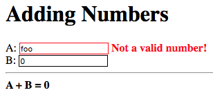
First let’s investigate more closely what happens when an invalid value is entered by the user. Let’s try it out with the sum application we wrote in Section 2, “Functional Bindings”.
You may have noticed that nothing happens if a number is only entered in one of the fields:
Let’s enter an invalid value for B, and see what happens:
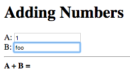
Again nothing. Is there something wrong with application?
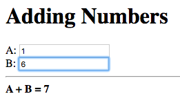
Let’s change B to a valid number:
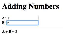
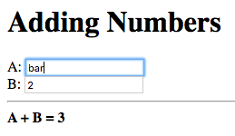
Now we get the result of the addition, 3. The application resumed
its normal operation when valid input is entered.
What will happen if we change one of the fields to an invalid value, let’s try changing A this time:
No change in the result of 3. It appears the application does not
change the result if invalid input was entered. This demands an
explanation.
What’s really going on under the hood is that when a value, which is not a valid number, is entered in one of the input fields, the node bound to that field is set to a failure value.
A failure value is a special type of value which, when evaluated, terminates the evaluation of the node, by which it was evaluated, and the node’s value is set to the failure value. Failure values represent the failure of an operation, the absence of a value or special classes of values.
In the sum application, a failure value is returned by the to-int
meta-node, when the argument is a string which does not contain a
valid integer. Thus to-int(a) evaluates to a failure value if the
value entered in the input field for A does not contain a valid
integer.
Remember that |
The observer of to-int(a) is a, and is thus set to the failure
value returned by to-int. Node a + b evaluates node a, thus
evaluating the failure value. This results in the computation of the
sum (a + b) being terminated and node a + b, and its observer
sum, being set to the failure value.
By default when a node, bound to a user interface element, evaluates to a failure value, the user interface is not updated. As a result the application appears to be doing nothing.
Whilst the current behaviour of the application is a step up from crashing or producing garbage results, it does not provide any indication to the user that the input entered was invalid. This is confusing to the user as the application appears to not be working properly. Proper error handling should be in place.
The core module provides a handy utility meta-node fails?, which
returns true if its argument node evaluates to a failure, and false
otherwise. This can be used to detect failures in our application and
display an appropriate error message.
A related utility meta-node |
We need to detect failures in the a and b nodes which are bound to
the values of the input fields for A and B, respectively. This can
be achieved using the expression fails?(a) for a and fails?(b)
for b.
We would like to display a message, indicating that the input entered
was invalid, next to the field where invalid input was entered. This
can be achieved using a case expression. The following is the case
expression for a:
case(
    fails?(a) : "Not a valid number!",
    ""
)
The case expression returns the constant string “Not a valid
number!”, if fails?(a) is true, that is a evaluates to a failure,
otherwise it returns the empty string. To display the error message
next to the field for A, we can simply place the entire case
expression in an inline node declaration, between <?@ ... ?>, next to
the field. We can do the same for B, substituting a with b, to
get an error indication for B as well.
That’s it we have added error handling to an existing application without having to make fundamental changes to our application logic. In-fact the addition of error handling was as simple as adding new UI elements.
Let’s try it out. Build and run the application and enter an invalid value in one of the input fields:
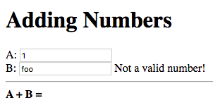
The message “Not a valid number!” is displayed next to the field containing the invalid value, B in this case.
Now correct the invalid value, to a valid number:
The message disappears and the sum is computed.
The error handling logic, added in the previous section, can do with some cleaning up.
- The error message is duplicated next to both fields. If we’d like to change the message we’d have to make sure we’ve changed it in both places.
-
The
caseexpression is identical for both fields with the only difference being the node. If we change the error handling logic, to display a different message, we’d have to edit both thecaseexpressions.
The case expression can be extracted into a
meta-node, let’s call it error-message which takes the node as input
and returns the appropriate error message.
Meta-Node error-message.
error-message(value) :
    case(
        fails?(value) : "Not a valid number!",
        ""
    )
Add this definition to the top of the Tridash code tag.
We can now replace the case expressions, inside the inline node
declarations with the following for field A:
error-message(a)
and the following for field B:
error-message(b)
Changes to the error message and error handling logic are now much
easier to implement as only the definition of the error-message
meta-node needs to be changed.
You may have noticed that the error messages are not displayed initially, when the input fields are empty. Similarly no visible result is observed until a value is entered in both fields. You’re probably wondering why this is so, as an empty string is certainly not a valid integer. In-fact, if you first enter a valid integer in a field, and then change its value to empty, the error message will be displayed.
The problem is that the nodes a and b are not given initial
values. As a result the value of the error-message(a) node, and the
corresponding node for b, is not computed until a is given its
first value. But then what happens when the node a + b is updated
after a value is entered in the first field, A, only? Since only the
dependency a, of a + b has been given a value, a + b does not
have a value for b and thus the value it uses for b defaults to a
failure. To solve this problem we can give initial values to a and
b.
An explicit binding in which the source is a literal constant and the target is a node is interpreted as giving the node an initial value, equal to the constant.
The following assigns an initial value of 1 to a and 2 to b:
Example.
1 -> a
2 -> b
The setting of the initial values is treated as an ordinary value
change from the default failure value to the given initial value,
which occurs immediately after the application is launched. As a
result, the values of the node’s observers are updated. In this case
the nodes: a + b, error-message(a) and error-message(b) will be
updated.
In our application, let’s give both a and b an initial value of
0. Add the following to the Tridash code tag at the top of the file:
0 -> a
0 -> b
Build and run the application:
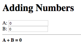
Both fields are initialized to 0 and the sum of 0 is
displayed.
Experiment with changing the node’s initial values and even try setting them to invalid integers.
You may be wondering how it is that giving an initial value to
the nodes |
As an exercise make the color of the border, or alternatively the background color, of the input element change to red when an invalid value is entered in it.
Try to achieve something similar to the following:
Some CSS styling rules have also been added to change the text color of the error messages to red, this is not part of the exercise. |
To change the border color of an element bind to the
|
The error handling tools we’ve seen so far have one serious shortcoming, there is no means for identifying the cause of the error. In the application, which we augmented with error handling in the previous tutorial, we don’t check at all what the cause of the failure is. Instead, we simply assumed that a failure value means invalid input was entered. Whilst this is the case in our simple application, it is not the case for more complex real world applications where there are many potential sources of errors.
Each failure value has an associated type, which is a value that
identifies the cause of the failure. The failure type can be
obtained using the fail-type meta-node from the core module. If
the argument of fail-type evaluates to a failure, the meta-node
returns its type, otherwise if the argument does not evaluate to a
failure or evaluates to a failure without a type, the meta-node
returns a failure.
The meta-node fail-type is a bit clunky to use as it, itself,
returns a failure if the argument does not evaluate to a failure
value. The utility fail-type? meta-node, also from the core
module, takes two arguments, a value and a failure type, and returns
true if the value evaluates to a failure of that type.
A value used as a failure type is generally bound to a constant node,
which is used in place of the raw value. An accompanying node, with
the same identifier but with a trailing ! is bound to a failure of
the type.
The type of the failure returned by to-int, when given a string that
does not contain a valid integer, is designated by the node
Invalid-Integer, from the core module. The node Invalid-Integer!
is bound to a failure of type Invalid-Integer.
We can use the fail-type? meta-node to explicitly check whether the
failure is of the type Invalid-Integer. Simply replace
fails?(value) with fail-type?(value, Invalid-Integer) in the
definition of the error-message meta-node.
Improved error-message Meta-Node.
error-message(value) :
    case(
        fail-type?(value, Invalid-Integer) : "Not a valid number!",
        ""
    )
The new implementation returns the string “Not a valid number!” only for errors caused by invalid input being entered. It returns the empty string for errors of any other type.
Failures are limited in use if they can only be created by builtin
meta-nodes. You can create your own failure values using the fail
meta-node, which takes one optional argument — the type of the
failure. If the type argument is not provided, a failure without a
type is created.
Example.
# Creates failure with no type
fail()

# Creates a failure with type `My-Type`
fail(My-Type)
Suppose for some reason, we’d like to limit the numbers being added, in the Adding Numbers application, to positive numbers. It could be that the numbers represent amounts for which negative values do not make sense in the context of the application.
Let’s write a meta-node, validate, which takes an integer value and
returns that value if it is greater than or equal to zero. Otherwise
it returns a failure of a user-defined type designated by the node
Negative-Number.
Meta-Node validate.
validate(x) :
    case(
        x >= 0 : x,
        fail(Negative-Number)
    )
If the argument x is greater than or equal to zero it is returned
directly, otherwise a failure, created using the fail meta-node, of
type designated by Negative-Number is returned.
Now let’s bind the Negative-Number node to a value, which uniquely
identifies the failure. For now let’s choose the value -1. While
we’re at it let’s also define the Negative-Number! meta-node which
is simply bound to a failure of type Negative-Number.
Failure Type `Negative-Number `.
Negative-Number  <- -1
Negative-Number! <- fail(Negative-Number)
We can simplify validate by substituting fail(Negative-Number)
with Negative-Number!:
Simplified validate Meta-Node.
validate(x) :
    case(
        x >= 0 : x,
        Negative-Number!
    )
It does not matter whether you place the binding declarations of
the nodes |
To incorporate this in our application, we have to change the nodes,
to which the input fields are bound, from a and b to input-a and
input-b.
Replace a with input-a, in the text field for A, and b with
input-b in the text field for B.
...
<label>A: <input value="<?@ to-int(input-a) ?>"/></label>
...
<label>B: <input value="<?@ to-int(input-b) ?>"/></label>
...
Also change the setting of initial values such that they are set on
nodes input-a and input-b rather than a and b.
0 -> input-a
0 -> input-b
Now we’re going to bind a to the result of validate applied on
input-a and we’re going to bind b to the result of validate
applied on input-b.
a <- validate(input-a)
b <- validate(input-b)
Finally let’s update the error-message meta-node to return “Number
must be greater than or equal to 0!” in the case that the failure
is of type Negative-Number.
Updated error-message Meta-Node.
error-message(value) :
    case(
        fail-type?(value, Invalid-Integer) :
            "Not a valid number!",
        fail-type?(value, Negative-Number) :
            "Number must be greater than or equal to 0!",
        ""
    )
Build and run the application and enter a positive number in one field and a negative number in the other:
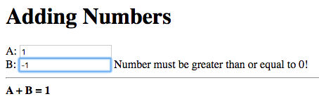
The error message, explaining that a positive number (or zero) must be entered, is displayed next to the field where the negative number was entered, B in this case. The result of the addition with the new numbers entered is not displayed, instead the previous result is retained, as expected.
Change the negative number to an invalid number:
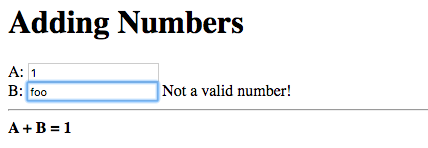
The error message changes to “Not a valid number!” and the displayed sum is unchanged, as in the previous versions.
Now change the value to a valid positive number:
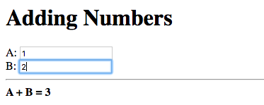
The error message disappears and the new sum is displayed.
There is one issue with the application we’ve just developed. There is
no guarantee that the arbitrary constant -1 uniquely represents a
failure of type Negative-Number. If all failure types used arbitrary
integer constants, there is no guarantee that -1 doesn’t already
represent a builtin failure type, such as Invalid-Integer. Whilst it
so happened to work, it is certainly not robust, especially when
bringing in third party libraries.
A value, which is guaranteed to be unique, can be obtained by taking a
reference to the raw node object of Negative-Number.
A reference to the raw node object, of a node, can be obtained using
the & special operator, which takes the identifier of the node as an
argument. Raw node references are mostly useful when writing macros,
which you’ll learn about in a later tutorial. For now all that you
need to know is that this value can serve as the failure type,
i.e. can be compared using =, and is guaranteed to be unique.
Replace the binding declaration for Negative-Number with the
following:
Proper Negative-Number Failure Type.
Negative-Number <- &(Negative-Number)
And now we have a robust way of distinguishing between failures
originating from to-int, due to the input fields not containing
valid integers, and errors originating from our own application logic.
Wow, we had to make so many fundamental changes to our code just to implement a minor change in the input accepted by the application. We had to:
-
Add the nodes
input-aandinput-b, for which we had to come up with meaningful identifiers. -
Change the input fields to be bound to
input-aandinput-brather thanaandb. -
Change the initial values to be assigned to
input-aandinput-brather thanaandb. -
Bind
atovalidate(input-a)andbtovalidate(input-b).
This is contrary to “simply adding new UI elements” which was the case when we introduced error handling. We can do better.
Notice that a lot of the code we added was simply repetitive binding
boilerplate code, which is the same for both a and b. It would be
nice if we could somehow abstract it away and not have to write the
same code for both nodes. Luckily, there is a way.
Remember, from the second tutorial, that some meta-nodes, such as
to-int, are special in that a two-way binding is established between
the meta-node instance and the argument node. This allows instances of
the meta-node to also appear as targets of bindings.
Refresher Example.
# The following
a -> to-int(b)

# Is equivalent to
to-int(a) -> b
It turns out to-int is not so special as we can do the same for our
own meta-nodes by setting the target-node attribute.
Node attributes are simply key-value pairs associated with a node,
which control various compilation options. Attributes are set using
the special /attribute operator:
/attribute Operator Syntax.
/attribute(node, key, value)
This sets the attribute of node with key key to the value value.
Examples.
# Set value of attribute `my-attribute` to 1
/attribute(a, my-attribute, 1)

# Set value of attribute `akey` to literal symbol `raw-id`
/attribute(b, "akey", raw-id)
|
Node attributes do not form part of a runtime node’s state. |
The target-node attribute determines, when set, the meta-node which
is used as the binding function of the binding in the reverse
direction, from a meta-node instance to the meta-node arguments.
As an example, a meta-node f with its target-node attribute set to
g results in the following:
Example.
/attribute(f, target-node, g)

# The following
a -> f(b)

# Is equivalent to
g(a) -> b
In the example above the target-node attribute of f is set to
g. Thus the declaration f(b) also results in the binding g(f(b))
-> b being created.
The meta-node to-int simply has its target-node attribute set to
itself, which is why it performs the same function, when it appears as
the target of a binding, as when it appears as the source of a
binding.
The |
Our code can be simplified considerably by allowing a meta-node, which
performs the additional input validation, to be bound (as the target)
to the values in the input field. Let’s first write that meta-node,
called valid-int which is responsible for converting an input string
to an integer and ensuring that the resulting integer is greater than
or equal to zero. In essence this meta-node combines to-int, we’ll
use int this time, and validate.
Meta-node valid-int.
valid-int(value) : {
    x <- int(value)
    validate(x)
}
In order to allow the node to appear as the target of a binding, and
still perform the same function, let’s set its target-node attribute
to itself:
/attribute(valid-int, target-node, valid-int)
Now we can bind the contents of the input fields directly to an
instance of the valid-int meta-node. In-fact, we can place the
valid-int instance directly in an inline node declaration.
Replace to-int(input-a) with valid-int(a), and the same for b,
in the input fields as follows:
<label>A: <input value="<?@ valid-int(a) ?>"/></label>
<label>B: <input value="<?@ valid-int(b) ?>"/></label>
The nodes input-a and input-b can be removed, as well as the
following declarations:
 a <- validate(input-a)
 b <- validate(input-b)
The initial values of 0 can once again be given to the nodes a and
b rather than input-a and input-b.
 0 -> a
 0 -> b
The following is the full content of the Tridash code tag.
/import(core)

# Error Reporting

error-message(value) :
    case(
        fail-type?(value, Invalid-Integer) :
            "Not a valid number!",
        fail-type?(value, Negative-Number) :
            "Number must be greater than or equal to 0!",
        ""
    )

# Input Validation

Negative-Number  <- &(Negative-Number)
Negative-Number! <- fail(Negative-Number)

validate(x) :
    case(
        x >= 0 : x,
        Negative-Number!
    )

valid-int(value) : {
    x <- int(value)
    validate(x)
}

/attribute(valid-int, target-node, valid-int)

# Initial Values

0 -> a
0 -> b
Compared to the previous version, the only modifications are in the
error-message meta-node, the inline bindings in the input fields and
the addition of the validate and valid-int meta-nodes along with
the Negative-Number failure type. This version, however, did not
require the addition of new nodes or modifying the bindings comprising
the core application logic. Changing the input validation logic was
simply a matter of substituting to-int with valid-int in the
bindings to the input field values.
Throughout these tutorials, we’ve glossed over two-way bindings without going into much detail of how they work, yet they were a vital component of every application as the bindings to the UI elements have all been two-way bindings.
Each node has a number of contexts which store information about how to compute the node’s value, i.e. what function to use and what dependencies are operands to the function. The active context of a node, at a given moment in time, is the context which is used to compute the node’s value. In general, a context is activated when the value of an operand node of the context changes. By default, a node context is created for each dependency of a node which was added by an explicit binding.
Example.
a -> x # Context created for dependency `a`
b -> x # Context created for dependency `b`
c -> x # Context created for dependency `c`
In this example node x has three contexts one for each of its
dependency nodes, a, b and c, to which it is bound explicitly.
An implicit binding between a meta-node instance and the meta-node arguments does not result in the creation of a context for each operand.
a + b
Nodes a and b are implicitly added as dependencies of a + b
however they are added as operands to the same context with the +
function.
The following application demonstrates how different contexts are activated, when the values of their operand nodes change.
ui.html.
<?
 x -> node
 y -> node
 z -> node
?>
<!doctype html>
<html>
    <head>
        <title>Node Contexts</title>
    </head>
    <body>
      <div><label>X: <input value="<?@ x ?>"/></label></div>
      <div><label>Y: <input id="b" value="<?@ y ?>"/></label></div>
      <div><label>Z: <input value="<?@ z ?>"/></label></div>
      <hr/>
      <div><strong>Last value entered: <?@ node ?></strong></div>
    </body>
</html>
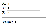
This is a simple application consisting of three text input fields
bound to nodes x, y and z. Nodes x, y and z are each
explicitly bound to node, the value of which is displayed below the
fields.
Let’s enter a value in each field and see what happens. Observe the value displayed below the fields after each change:
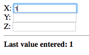
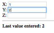
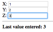
Notice that after each change, the value that was just entered is displayed.
Now let’s try changing the values of the fields which were edited previously:
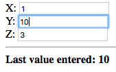
In this case the value of the second field, Y, was changed to 10 and that value was immediately displayed below the fields.
The value of the field that was changed last is displayed. To understand why this is so, let’s examine the sequence of steps taken when a value is entered in the X field.
-
The value of
x, which is bound to the value in the X field, is updated. -
The context corresponding to the binding
x -> nodeis activated due to the value ofxbeing updated. -
The value of
nodeis updated to the value ofx.
Contexts make two-way bindings possible:
Example.
input1 -> a

# Two-way binding
a -> b; a -> b

input2 -> b
The |
a has two contexts corresponding to dependency nodes input1 and
b (which is also an observer). b has two contexts corresponding to
dependency nodes input2 and a.
When input1 is changed, the contexts corresponding to the bindings
in the following direction are activated:
-
input1 -> a -
a -> b
When input2 is changed, the contexts corresponding to the bindings
in the following direction are activated:
-
input2 -> b -
b -> a
The context of a binding can be set explicitly to a named context,
using the @ operator from the core module.
a -> b @ context-id
The binding a -> b is established in the context, of b, with
identifier context-id.
When multiple bindings are established to the same explicit context, the observer node takes on the value of the first operand which does not evaluate to a failure. The operands are ordered by the order in which the explicit bindings are declared in the source file. If all the operands evaluate to failures, the node evaluates to the failure value of the last operand.
This is better explained with an example application:
ui.html.
<?
 /import(core)

 x -> node @ context
 y -> node @ context
 z -> node @ context
?>
<!doctype html>
<html>
    <head>
        <title>Explicit Contexts</title>
    </head>
    <body>
      <div><label>X: <input value="<?@ to-int(x) ?>"/></label></div>
      <div><label>Y: <input value="<?@ to-int(y) ?>"/></label></div>
      <div><label>Z: <input value="<?@ to-int(z) ?>"/></label></div>
      <hr/>
      <div><strong>Value: <?@ node ?></strong></div>
    </body>
</html>
This application is similar to the previous application except the
bindings from nodes x, y and z, to node are established in an
explicit context with identifier context. Additionally the input
fields are bound to to-int instances, of x, y and z which
results in x, y and z being bound to the values entered in the
fields converted to integers. If a non-integer value is entered in a
field, the corresponding node is bound to a failure value.
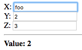
Let’s try it out. Enter some integer values in each of the fields:
The value entered in the first field, X, was displayed. Since a
valid integer was entered, node x evaluates to the integer value
1. The binding x -> node was established first, as the declaration
occurs first in the source file, and since x does not evaluate to a
failure, node takes on the value of x. The values of y and z
are ignored.
Now let’s change x to a non-integer value:
The value entered in the second field, 2, is displayed. Since a
non-integer value was entered in the first field, x evaluates to a
failure. node thus takes on the value of the next dependency, bound
to the explicit context, which does not evaluate to a failure. The
dependency is y which evaluates to the integer entered in the second
field, 2.
Let’s see what happens if we enter a non-integer value in the third field:
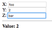
The displayed value is unchanged since the second dependency, node
y, already evaluates to a value which is not a failure value. The
value of the third dependency z, corresponding to the value entered
in the third field, is ignored, regardless of whether it evaluates to
a failure or not.
Explicit contexts are a useful tool for handling failures. In the previous application a failure originating from the first input field, was handled by taking the value of the node bound to the second field. Similarly a failure originating from the second input field is handled by taking the value entered in the third field.
The @ operator also allows a binding to be activated only if the
result of the previous binding(s), in the same context, is a failure
value with a given type. When the context identifier is of the form
when(context, type) the binding is only activated if the result of
the previous binding(s) is a failure of type type.
Example.
x -> node @ context
y -> node @ when(context, Invalid-Integer)
z -> node @ when(context, Negative-Number)
Three bindings to node are established in the explicit context
context.
node is primarily bound to the value of x if it does not evaluate
to a failure. If x evaluates to a failure of type Invalid-Integer,
node is bound to the value of y. If x, or y evaluate to a
failure of type Negative-Number, then node is bound to the value
of z.
To try this out replace the binding declarations, in the application
from the previous section, with the declarations in the example
above. Also copy over the definition of the meta-nodes valid-int,
validate and the Negative-Number failure type from
Section 8.3, “Target-Node for own Meta-Nodes”, into the Tridash code tag. Replace
to-int with valid-int in the inline node declarations within the
input field values.
Enter a non-integer value in the first field, and an integer value in the second and third fields:
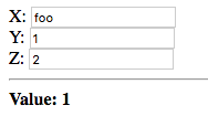
The value of the second field is displayed, since node is bound to
it when the value in the first field is not an integer.
Now change the value of the second field to a negative integer, or alternatively enter a negative integer value in the first field:
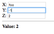
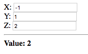
The value of the third field is displayed in both cases, even when the
value of the second field is a valid positive integer. This is due to
node being bound to the value of the third field when either the
value of the first field or second field is a negative number.
a -> b @ when(context, type) can be rewritten as: a -> b @ context when type |
Whilst the error handling logic in the Adding Numbers application,
from Section 8, “Target Node Transforms”, is adequate and correct, the
definition of the error-message meta-node, responsible for selecting
an appropriate error message, can be improved using explicit
contexts. The current definition repeatedly checks whether the failure
type of the value argument is of a given type using the fail-type?
meta-node. This is repetitive and does not convey the intent that this
is error handling/reporting logic.
The error-message meta-node returns:
-
The empty string if the
valueargument does not evaluate to a failure. -
The string “Not a valid number!” when
valueevaluates to a failure of typeInvalid-Integer. -
The string “Number must be greater than or equal to 0!” when
valueevaluates to a failure of typeNegative-Number.
We can re-implement this logic using bindings to the self node with
explicit contexts.
The self node should primarily be bound to the empty string, if the
value argument does not evaluate to a failure. There is a handy
utility meta-node, !-, in the core module, which returns the value
of its second argument if the first argument does not evaluate to a
failure. If the first argument evaluates to a failure value, it is
returned. This meta-node is registered as an infix operator thus can
be placed between its arguments.
The primary binding can thus be written as follows:
value !- "" ->
    self @ context
If this binding results in a failure of type Invalid-Integer, self
should be bound to the constant string “Not a valid number!”. This
is achieved with the following:
"Not a valid number!" ->
    self @ context when Invalid-Integer
Finally self should be bound to “Number must be greater than or
equal to 0!”, if the previous bindings resulted in a failure of type
Negative-Number.
"Number must be greater than or equal to 0!" ->
    self @ context when Negative-Number
Putting it all together we have the following definition of
error-message re-implemented using explicit contexts:
New implementation of error-message.
error-message(value) : {
    value !- "" ->
        self @ context

    "Not a valid number!" ->
        self @ context when Invalid-Integer

    "Number must be greater than or equal to 0!" ->
        self @ context when Negative-Number
}
The advantage of this implementation is that it more explicitly
conveys the intent that this is error handling logic. As such it can
be optimized more effectively, e.g. if self evaluates to a failure
of type Negative-Number, the check for whether the failure type is
Invalid-Integer can be skipped altogether.
An additional advantage of this implementation is that the third
binding is activated on failures of type Negative-Number originating
both from the first and second bindings whereas the previous
implementation only handled failures originating in value. In this
case it doesn’t make a difference as the second binding cannot result
in a failure of type Negative-Number. However this does make a
difference, in more complex error handling logic, where the handling
of an error may itself result in a new error.
This implementation does, however, have a difference from the previous
implementation in that if value evaluates to a failure of a type
other than Invalid-Integer or Negative-Number it returns a
failure, whereas the previous implementation returned the empty
string. In this application it doesn’t make a difference as the
arguments passed to error-message do not evaluate to failures of
other types.
Coming up with a context identifier and typing it out repeatedly can become tiresome. The original reason for having an identifier for explicit contexts is to distinguish them from the remaining contexts which are implicitly created and to allow for multiple explicit contexts. However, there is usually only a single explicit context used for handling failures.
To shorten the syntax for binding to an explicit context, a default
identifier, such as _ can be given to all explicit contexts which
are used only for handling failures. Alternatively, the @ operator
can take a single argument, the node, in which case it is a shorthand
for the explicit context with identifier default.
# The following:
x -> y @ default

# Is equivalent to:
x -> @(y)
When the context identifier is of the form when(type), that is
omitting the context identifier and leaving only the failure type, the
explicit context with identifier default is, once again, assumed.
# The following:
x -> y @ default when type

# Is equivalent to:
x -> y @ when(type)
So far, we’ve seen that Tridash is good at producing an output, which is a function of a given input, and ensuring that it is always synchronized with the input. What we haven’t seen, however, is mapping a previous output to a new output. In-fact, with the tools introduced so far, this is impossible.
To be able to map a previous output to a new output, a binding has to be established in which the source is a function of the target node. As an example, to implement a counter, intuitively we might do the following:
# This does not work!!!
counter + 1 -> counter
The problem here is that a change in the value of counter triggers a
change in the value of counter, which triggers a further change in
the value of counter ad infinitum. What we require is a way to
tell Tridash, that when the value of counter is updated to counter
+ 1, it should not trigger another update to the value of counter +
1. We also need a way to specify when we would like the value of
counter to be updated to counter + 1, as updating it only once is
hardly useful.
Node states allow us to control when the value of a node is updated,
beyond the simple rule of whenever the value of one of its dependency
nodes changes. The target of a binding can have an explicit state
associated with it, using the :: operator. In this case the binding
is referred to as a stateful binding.
Explicit state using :: operator.
a -> b :: state-id
The left-hand side of the :: operator is the node and the right hand
side is the state identifier, which is a symbol identifier (similar to
a context identifier). The result of this is that the binding a -> b
only takes effect when b switches to the state with identifier
state-id. The emphasis is on switches as a change in the value of
a will not automatically trigger a change in the value of b. Only
a change in the state of b will trigger a change in its
value. This may seem counter-intuitive at first, however if b was
updated on every change in the value of a, and instead of a we
have b + 1 we’ll end up with the same problem, as in the previous
section.
Stateful bindings declared later in the source take priority over those declared earlier. |
A node’s state is determined by the value of the special node
/state(node). Binding to it allows us to control a node’s state.
Example: Counter.
counter + 1 -> counter :: increment
/state(counter) <-
case(
should-increment? : '(increment),
'(default)
)
The |
In this example, a binding counter + 1 -> counter is established
which only takes effect when counter switches to the increment
state.
The second declaration binds a case expression to the
/state(counter) node, thus controlling the state of counter. When
should-increment? is true the value of the case expression, and
thus the state of counter is increment, otherwise it is default.
The result is that when the value of /state(counter) (the state of
counter) is updated to increment, the value of counter is
updated to it’s previous value incremented by 1.
To provide a runnable example, we have to interface with JavaScript in order to hook into its event system. In the next major release of Tridash, this wont be necessary.
This section will go over only the basics of interfacing with JavaScript, which are necessary for completing this tutorial. A full in-depth tutorial on interfacing with JavaScript, will follow.
Tridash nodes are compiled to runtime node objects, which store the
node’s value. To be able to reference a runtime node object from
JavaScript, the node has to be given an identifier with which it can
be referenced. The public-name attribute, if given, determines the
name of this identifier.
Once an identifier is given, it can be accessed as a member of the
nodes property of the runtime module object. To access the runtime
module object of a compiled Tridash program, embedded in an HTML file,
it needs to be given an identifier. The module is then accessible via
a global variable with that identifier. This is achieved using the
module-name output options.
Currently Tridash does not check whether multiple nodes are
given the same |
Example: Setting public-name identifier.
/attribute(node, public-name, "aNode")
Example: Referencing the runtime node object in JavaScript.
// Assuming runtime module is stored in variable mod var node = mod.nodes["aNode"]; // or equivalently if the public-name is a valid JS variable name var node = mod.nodes.aNode;
Once a reference is obtained to the runtime node object, the node’s
value can be set using the set_value method, which takes the value
as an argument.
Example: Setting Node Value from JavaScript.
node.set_value(1);
It is important, however, that if set_value will be called on a
runtime node object, the node is marked as an input node, by setting
its input attribute to true.
/attribute(node, input, True)
Not every Tridash node corresponds to an actual runtime node object, due to some intermediate nodes being optimized out by the compiler. The only nodes, for which it is guaranteed that a runtime node object is created, are input nodes and nodes with no observers, which are assumed to represent output nodes. |
In this section we’ll build a very simple application consisting of a counter which is incremented when a button is pressed.
Let’s start off with the Tridash binding declarations. We’ve in-fact already written the bulk of the code in the previous example, which we can simply copy into our new application.
counter + 1 -> counter :: increment
/state(counter) <-
case(
should-increment? : '(increment),
'(default)
)The node counter stores the value of the counter which is
incremented when should-increment? is true. We’ll add the attributes
which are necessary in order to be able to set the value of
should-increment? from JavaScript, namely we need to set the
public-name identifier and mark it as an input node.
/attribute(should-increment?, input, True)
/attribute(should-increment?, public-name, "should_increment")
We’ll allow the user to set/reset the value of the counter by binding
a start node to an input field. We’ll bind start directly to
counter and give it an initial value of 0.
start -> counter
0 -> start
Now let’s define the user interface. We need a text input field for
entering the initial value for the counter, which will be bound to
start and an increment button. The value of the counter will be
displayed below the counter.
ui.html.
...
<div><label>Start: <input value="<?@ to-int(start) ?>"/></label></div>
<div><button id="increment">Increment</button></div>
<hr/>
<div><strong>Counter: <?@ counter ?></strong></div>
...
The HTML boilerplate is not shown. |
We’ve given the Increment button the ID increment so that we can
attach an event listener to its click event. We’ll do so using the
following JavaScript code, in a script tag which should be added below
the element where the counter is displayed:
<script>
  document.addEventListener("DOMContentLoaded", async () => {
      const module = await mod;

      const increment = document.getElementById('increment');
      const node_increment = module.nodes.should_increment;

      increment.addEventListener('click', function() {
          node_increment.set_value(true);
          node_increment.set_value(false);
      });
  });
</script>
A couple of things to note:
-
We’ve assumed the runtime module object is stored in the global
variable
mod. The runtime module object identifier will be set with themodule-nameoutput option. -
The entire code is wrapped in an event handler for the
DOMContentLoadedevent to ensure that it is run after the JavaScript code which assigns the runtime module object tomod. -
awaitis applied on the module objectmod, inside anasynccallback function, since the module itself may be created asynchronously. This is the case when the compilation target is WebAssembly (wasm32).
The callback function, run after all HTML elements and scripts have been loaded, does the following:
-
Obtains a reference to the HTML element with ID
increment. -
Obtains a reference to the
should-increment?node which was given apublic-nameofshould_increment.
The remainder of the function attaches a listener, for the click event,
on the Increment button. In that listener we first set the value of
the should-increment? node to true, then immediately afterwards we
set it to false again.
Setting the value of should-increment? to true, causes the state of
counter to change to increment. Setting it back to false again
causes the state to change to default.
In a future release, when the HTML library is complete, a
subnode |
Change the build configuration file (build.yml) to the following:
build.yml.
sources:
  - path: ui.html
    node-name: ui

output:
  path: app.html
  type: html
  main-ui: ui
  module-name: mod
The addition of the line module-name: mod sets the module-name
output option to mod, which is the identifier of the variable in
which the runtime module object will be stored.
Build and run the application, and press the increment button a few times:
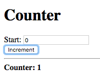
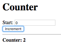
The displayed value, for the counter, is incremented after each press.
Now enter a value in the Start field to reset the counter, and then press the increment button again:
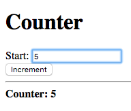
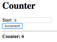
The counter is reset to the value entered in the Start field. Pressing increment afterwards increments the new counter value.
Let’s do a little experiment, comment out the line, in the click event handler, which sets the value of the should-increment? node to false, i.e. comment out the following:
node_increment.set_value(false);
What do you expect to happen? Initially, we might think that since the
should-increment? node is not being reset to false, the state of
counter is not being reset to default. The state of counter will
thus switch to increment once, after which, there are no further
state changes. The result is that the counter will only be incremented
the first time the increment button is pressed.
Let’s try it. Build and run the application and press the increment button twice.
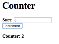
What happened? The counter carries on incrementing after the first button press. Why?
The declaration:
counter + 1 -> counter :: increment
states that the binding should only take effect when the state of
counter switches to the increment state. Switching from the
increment state to the increment state is still considered as
switching to the increment state, even though the new state is
identical to the previous state. This is due to the fact that each
time we’re setting the value of the should-increment? node to
true, we’re triggering a change in the value of the node
/state(counter) and thus the state of counter, even though the new
value of should-increment? is identical to its previous value.
The above declaration should thus be thought of as declaring a binding
which takes effect whenever counter switches from any state,
including increment, to the increment state.
To fix this issue we can specify an explicit from state. When specified, the binding only takes effect when the state of the node changes from the from state to the to state. This is specified using the following syntax:
Node State Binding with Explicit From State.
a -> b :: previous => next
When the state identifier is a functor of the form previous => next,
previous is interpreted as the identifier of the from state and
next is interpreted as the identifier of the to state.
To achieve the intuitive behaviour we can limit the binding counter +
1 -> counter to only take effect when the state of counter
transitions from default to increment. Replace the binding
declaration of counter with the following:
counter + 1 -> counter :: default => increment
This implementation will, however, require two initial button presses
before the counter starts incrementing. This is due to the fact that
we haven’t given counter an initial state. The first press causes it
to change to increment, and then back to default, however since it
is not a change from default to increment, the binding does not
take effect. We can fix this by giving /state(counter) an initial
value of default.
Setting Initial State.
'(default) -> /state(counter)
Now the counter starts incrementing after the first press.
Let’s repeat the experiment on this new implementation, comment out
the line, in the JavaScript script tag, which sets the value of
should-increment? to false. The counter should only increment the
first time the Increment button is pressed.
This example served to demonstrate the difference between a stateful binding with and without a from state. However, in this example, there is no value in specifying a from state, as the previous example, without a from state, was simpler and performed the same function.
In this example, we’ll build a silly application in which the Increment button, the button which actually increments the counter, alternates between two buttons. The goal of this example is to demonstrate what can be done with stateful bindings with a from state that cannot be done with stateful bindings without a from state.
We’ll start off with a similar interface to the previous counter application, however with two increment buttons.
ui.html.
<h1>Counter</h1>
<div><label>Start: <input value="<?@ to-int(start) ?>"/></label></div>
<div>
  <button id="increment1">Increment 1</button>
  <button id="increment2">Increment 2</button>
</div>
<hr/>
<div><strong>Counter: <?@ counter ?></strong></div>
Both button’s have been given ID’s as we’ll need to attach event listeners to both buttons, in JavaScript.
We’ll need two nodes clicked1? and clicked2? which change to true
when the first and second buttons are clicked, respectively. The
values of these nodes will have to be set via JavaScript, thus we’ll
mark them as input nodes and set their public-name attributes:
/attribute(clicked1?, input, True)
/attribute(clicked1?, public-name, "clicked1");

/attribute(clicked2?, input, True)
/attribute(clicked2?, public-name, "clicked2");
The following JavaScript code attaches event listeners for the clicked events, of both buttons, which simply set the value of the corresponding clicked? node to true and them immediately to false, again.
document.addEventListener("DOMContentLoaded", async () => {
    const module = await mod;

    const increment1 = document.getElementById('increment1');
    const increment2 = document.getElementById('increment2');

    const clicked1 = module.nodes.clicked1;
    const clicked2 = module.nodes.clicked2;

    increment1.addEventListener('click', function() {
        clicked1.set_value(true);
        clicked1.set_value(false);
    });

    increment2.addEventListener('click', function() {
        clicked2.set_value(true);
        clicked2.set_value(false);
    });
});
We’ll need two states for the counter node:
-
increment1 - Corresponds to the first button being clicked last.
-
increment2 - Corresponds to the second button being clicked last.
The value of counter should be incremented only when its state
switches from one state to the other, i.e. the button, which was
clicked, is different from the previous button to be clicked. This can
be achieved using two stateful bindings which take effect during the
state transitions increment1 => increment2, increment2 =>
increment1.
counter + 1 -> counter :: increment1 => increment2
counter + 1 -> counter :: increment2 => increment1
|
counter will retain its previous value during any other state
transition.
We need to set counter's state, to increment1 or
increment2, based on which button was clicked last. To achieve that
we can exploit the fact that each explicit binding to a node, without
an explicit context, results in the creation of a new context. When
the value of the source node, of the binding, changes, the binding
context is activated.
We know that the value of clicked1 changes to true, and then to
false, again, when the first button is clicked. The same is true for
clicked2 when the second button is pressed. We want the state of
counter (/state(counter)) to be bound to the literal symbol
increment1, when the value of clicked1 changes regardless of what
that value is. For that, we can use the utility !- meta-node,
introduced in Section 9.3, “Improved Error Handling in Adding Numbers”, which
returns the value of its second argument if its first argument does
not evaluate to a failure.
The following are the binding declarations which set the state of
counter.
clicked1? !- '(increment1) -> /state(counter)
clicked2? !- '(increment2) -> /state(counter)
The sole purpose of the |
To make it obvious which button should be clicked, we’ll make the
button which increments the counter change to green. We’ll bind each
button’s background color to "green" if the other button was the
last button to be pressed, and "gray" if it was the last button to
be pressed. This is achieved with the following:
increment1 <- /state(counter) = '(increment1)
increment2 <- /state(counter) = '(increment2)

case (increment2 : "green", "gray") ->
    self.increment1.style.backgroundColor
case (increment1 : "green", "gray") ->
    self.increment2.style.backgroundColor
We’re comparing the state of counter directly to determine which button was pressed last. |
Finally, let’s make the initial state of counter, increment2 so
that pushing on the first button, increments the counter.
Build and run the application. Initially you should see something similar to the following:
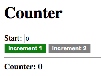
Click on the green Increment 1 button:
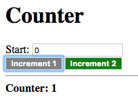
The counter is incremented by one, and the button changes to grey with the other button changing to green. Clicking on the same, now grey, button will not affect the value of the counter.
Click on the green Increment 2 button:
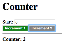
The counter is incremented once again, and button Increment 1 changes back to green with button Increment 2 changing back to grey.
Just to make sure everything works properly let’s reset the counter and push the green button to increment it.
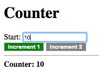
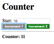
Everything works as expected. The state of counter does not affect
the binding start -> counter as it is a stateless, without an
explicit state specified, binding.
This tutorial is an introduction to processing lists of data. Lists
are conceptually represented as a linked list of nodes in which the
head of the node stores the list element and the tail stores the
next node, i.e. the remainder, of the list. The meta-nodes head and
tail, from the core module, return the head and tail of a list
node respectively.
This is only a conceptual view as not all lists are necessarily implemented as linked lists. Some lists are actually implemented as contiguous arrays which provide a linked list interface. In the current release, only linked lists can be created explicitly, however functionality for creating arrays will be added in a future release. |
The empty list is represented by the value of the node Empty. The
tail of the last node in a list is bound to this node.
The node |
The cons meta-node creates a list node, taking the value for the
head and the tail as arguments. This can be used to append to the
front of an existing list:
# Create a list of 1 element, by appending to the front of the empty
# list
l1 <- cons(a, Empty)

# Append to front of l1, creating a list of 2 elements
l2 <- cons(b, l1)
The list meta-node takes a variable number of arguments and returns
a list containing the values of the arguments as elements.
# Create list with elements: 1, 2, 3
l <- list(1, 2, 3)
The list* meta-node, also taking a variable number of arguments, is
used to prepend a number of elements to the front of a list. The last
argument is interpreted as a list with the remaining arguments
prepended to the front of it.
# Create list with 1 and 2 prepended to the front of l1
l2 <- list*(1, 2, l1)
Meta-Nodes can be passed to other meta-nodes as arguments, or bound to ordinary nodes, in which case the function of the meta-node is referenced.
A node can appear as the operator in a functor node in which case the function, of which the reference is stored in the node’s value, is applied on the arguments. If the node’s value is not a reference to function or the function is applied on an incorrect number of arguments, the result is a failure value.
Example.
call(f, arg) : f(arg)
func(x) : x

f <- func
result <- call(f, y)
In this example the call meta-node takes two arguments and returns
the result of applying the first argument f on the second argument
arg. The node f is bound to a reference to the function of the
meta-node func, which is then passed to the call meta-node.
An interesting aspect of higher-order programming in Tridash is that when referencing a meta-node as a value, which references the values of nodes declared in the global scope, a binding is established between the referenced nodes and meta-node reference. A binding is also established between the default values of optional arguments, in the case that they are references to other nodes, and the meta-node reference.
Example.
# Increment `x` by the value of the global node `delta
increment(x) : x + delta

call(f, arg) : f(arg)

result <- call(increment, n)
The increment meta-node references the value of the global delta
node. The function of the increment meta-node is referenced by the
node call(increment, n), thus a binding is established between
delta and call(increment, n). The result is that whenever the
value of delta is changed, the value of call(increment, n) is
updated.
Let’s demonstrate this with a simple application. Create a ui.html
file containing the above code in a Tridash code tag and the following
interface in the HTML body.
<div><label>N:<br/><input value="<?@ to-int(n) ?>"/></label></div>
<div><label>Delta:<br/><input value="<?@ to-int(delta) ?>"/></label></div>
<hr/>
<div>Result: <?@ result ?></div>
Build and run the application and enter a value for N and Delta.
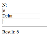
The result of the value entered for N plus Delta is displayed, nothing new here.
Now change the value for Delta:
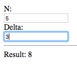
The result is updated even though there is no direct instance of
increment but rather a reference to the function of increment,
which is passed to the call meta-node. This demonstrates that an
implicit binding delta -> call(increment, n) is created due to
increment referencing the value of delta in its definition.
Higher-order meta-nodes are extremely useful for processing
lists. There are many list processing utility meta-nodes, in the
core module, which take a reference to a meta-node as an argument,
and perform an operation on the list using the meta-node. Here are few
examples:
map(f, list). The map meta-node takes a function f and a list as arguments and
returns a new list with the result of the applying the function on
each element of the list.
Example: map.
l <- list(1, 2, 3)

1+(n) : n + 1
map(1+, l)    # Result: list(2, 4, 6)
The meta-node 1+ returns its argument plus one. 1+ is applied on
each element of list l, containing the elements 1, 2, 3, using the
map meta-node. The result is the list containing the elements 2, 4,
6, which is each element of the original list plus one.
foldl(f, list). The foldl meta-node reduces a list to a single value by
applying a function on the first two elements of the list, and then
applies the function again on the result of the previous application
and the next element. This is repeated until there are no more
elements in the list.
Example: foldl.
l <- list(1, 2, 3)
foldl(+, l)  # Result ((1 + 2) + 3) = 6
In this example the + function is applied on the list containing the
elements 1, 2, 3. foldl first applies + on the first two elements
of the list (1, 2) producing the result 3. The + function is then
applied on the result 3 and the next element of the list 3, producing
the result 6.
The foldl'(x, f, list) function is similar to foldl except the
function f is first applied on x and the first element of the
list, rather than the first two elements of the list.
The foldr(f, list) function is similar to foldl except the
reduction starts from the last two elements of the list and proceeds
backwards until the first element.
Some other useful functions are:
-
filter(f, list) -
Returns a list containing only those elements of
listfor whichfreturns true. -
every?(f, list) -
Returns true if
freturns true for every element oflist. -
some?(f, list) -
Returns true if
freturns true for at least one element oflist. -
not-any?(f, list) -
Returns true if
freturns false for all elements oflist. -
not-every?(f, list) -
Returns true if
freturns false for at least one element oflist.
We’ll create a simple application consisting of an input field and an Add Message button. When the Add Message button is pressed, the message entered in the input field is appended to the list of messages, which are displayed below the button.
Start off with the following user interface:
ui.html.
<div><label>New Message: <input value="<?@ new-message ?>"/></label></div>
<div><button id="add">Add Message</button></div>
<hr/>
<pre><?@ messages ?></pre>
The value of the New Message input field is bound to the node
new-message. The value of the messages node is bound to the
contents of a pre tag. This node will store the list of messages in
a single formatted string.
The button is given the id add so that we can attach an event
listener for its click event, in JavaScript:
Add the following code, which is similar to the code seen in
Section 10, “Node States”, to a script tag below the pre tag:
document.addEventListener("DOMContentLoaded", async () => {
    const module = await mod;

    const add = document.getElementById('add');
    const clicked = module.nodes.clicked;

    add.addEventListener('click', function() {
        clicked.set_value(true);
        clicked.set_value(false);
    });
});
The value of the node with the public identifier clicked, which is
the add-clicked? node, is set to true and the immediately to false
when the button is clicked. Add the following attribute declarations
for the add-clicked? node:
/attribute(add-clicked?, input, True)
/attribute(add-clicked?, public-name, "clicked")
We’ll need a node to store the list of messages. Let’s call it
message-list and set its initial value to the empty list.
message-list <- Empty
The new message entered, bound to new-message, has to be added to
the end of message-list. The append meta-node takes two lists and
appends the second list at the end of the first list. Thus to append a
single item, we’ll pass a list of that one item to append.
append(message-list, list(new-message))
We want the value of new-message to be appended to message-list
when the Add Message button is clicked. This can be achieved with a
stateful binding to message-list in the add-new state.
append(message-list, list(new-message)) ->
    message-list :: add-new
The state of message-list should be set to add-new when the Add
Message Button is pressed. The add-clicked? node is true when the
button is being pressed and false otherwise, thus the state of
message-list can be set with the following case expression:
case(
    add-clicked? : '(add-new),
    '(default)
) -> /state(message-list)
We have completed the functionality for adding a message to the end of the messages list. All that remains is to format that list into a string which is displayed to the user.
We need a single string containing each message followed by a
newline. We’ll write a format-message meta-node which appends a line
break to a message.
Meta-Node format-message.
format-message(message) :
    format("%s\n", message)
format-message uses the format meta-node, introduced in
Section 4, “Writing your own Functions”, to produce a string containing the message, replacing
the %s placeholder, followed by a line break.
|
To format each message, we’ll apply format-message on each message
in message-list using map.
formatted-messages <- map(format-message, message-list)
Finally, to concatenate the formatted messages into a single string,
we’ll use the string-concat meta-node, which takes two strings as
arguments and returns the concatenation of both strings. We’ll need to
apply string-conat on each element in formatted-messages in turn,
accumulating the result in a single string. We can do that using the
foldl node, passing in string-concat as the reduction function:
messages <- foldl(string-concat, formatted-messages)
The resulting string is bound to messages which is displayed in the
pre (preformatted) tag, below the Add Message button.
Build and run the application, using the build configuration file from Section 10.3, “Example: Counter Application”. Enter a message and press the Add Message button.
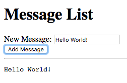
The message is displayed.
Now enter a new message and click the Add Message button.
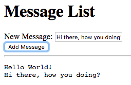
The message is displayed below the old message.
Up till this point we haven’t given much thought as to how our source
code is organized. Instead we’ve crammed all our code in a Tridash
code tag inside a single ui.html file. This strategy obviously wont
scale for larger applications. Ideally we’d like to have separation
of concerns with our application divided into multiple source files,
each containing the code implementing a separate component of the
application. The ui.html should ideally contain a minimal amount of
Tridash code, limited only to inline node references and bindings
directly related to the presentation logic. The core application logic
should be in a separate source file.
In this tutorial we’ll take the Adding Numbers application, as it is at the end of Section 9, “Contexts”, and reorganize its source code.
The simplest form of code organization is splitting up the application
into multiple source files. Source files containing only Tridash code
are given the extension trd.
Let’s extract the validation logic in a separate validation.trd
file. This includes the meta-nodes validate, valid-int and the
Negative-Number failure type.
validation.trd.
/import(core)

Negative-Number  <- &(Negative-Number)
Negative-Number! <- fail(Negative-Number)

validate(x) :
    case(
        x >= 0 : x,
        Negative-Number!
    )

valid-int(value) : {
    x <- int(value)
    validate(x)
}

/attribute(valid-int, target-node, valid-int)
We’ve kept the |
The application logic simply consists of the definition of the
error-message meta-node, which is responsible for choosing an
appropriate error message, the computation of the sum, and the setting
of the initial values for a and b.
Let’s place this in a separate source file called app.trd
app.trd.
/import(core)

error-message(value) : {
    value !- "" ->
        @(self)

    "Not a valid number!" ->
        self @ when(Invalid-Integer)

    "Number must be greater than or equal to 0!" ->
        self @ when(Negative-Number)
}

sum <- a + b

0 -> a
0 -> b
We’ve kept the |
We’ve bound the sum of |
All that’s left in the ui.html file is the user interface elements
and the inline bindings to the nodes a, b, sum and the
error-message instances, which display the error messages.
ui.html.
<!doctype html>
<html>
    <head>
        <title>Adding Numbers</title>
    </head>
    <body>
      <h1>Adding Numbers</h1>
      <div>
        <label>A: <input id="a" value="<?@ valid-int(a) ?>"/></label>
        <?@ error-message(a) ?>
      </div>
      <div>
        <label>B: <input id="b" value="<?@ valid-int(b) ?>"/></label>
        <?@ error-message(b) ?>
      </div>
      <hr/>
      <div><strong>A + B = <?@ sum ?></strong></div>
    </body>
</html>
To build an application consisting of multiple source files, the
source files are simply listed, under the sources entry, of the
build configuration file. Modify the build.yml file to the
following:
build.yml.
sources:
  - validation.trd
  - app.trd
  - path: ui.html
    node-name: ui

output:
  path: app.html
  type: html
  main-ui: ui
The source files are processed in the order they are listed. |
Since there are no processing options for validation.trd and
app.trd, we’ve listed the paths to the files directly rather than in
the path entry of a dictionary.
To build entirely from the command-line, simply list the files, in the
order they are to be processed, after The following is equivalent to the build configuration file tridashc validation.trd app.trd path : node-name=ui.html \
-o path.html -p type=html -p main-ui=ui |
Whilst separating the application into multiple source files, grouping
related components in a single file, is a significant cleanup, it
would be even better if the nodes could be grouped into different
namespaces based on their purpose, for example utility, application
logic and ui. This would allow us to use only the nodes from the
utility namespace, without having the rest of the utility nodes
clash (i.e. have the same identifiers) with the application logic
nodes. Whilst in this application there are no clashes, keeping the
nodes in separate namespaces allows us to use the same
validation.trd file in another application without the fear that
some node is going to clash with other nodes in the application.
Modules are a means of separating nodes into different namespaces,
where each module is a namespace in which nodes are contained. A node
with identifier x in module mod1 is a distinct node from the node
x in mod2, even though the two nodes share the same identifier.
We’ve already made use of the |
Modules are created with the /module operator which has the
following syntax:
/module Operator Syntax.
/module(module-name)
This indicates that all node references, in the declarations following
the /module declaration, will occur in the module with identifier
module-name. Remember that nodes are created the first time they are
referenced, thus if a node is referenced which is not in the module,
it is created and added to the module.
Example.
/module(mod1)
x -> node1

/module(mod2)
x -> node2
The first reference to the node x occurs in module mod1 thus a
node x is added to mod1. The second referenced occurs in module
mod2 thus the node is added to mod2. The two nodes are distinct
even though they share the same identifier.
If no module is specified the node references occur in a nameless init module. The current module is reset to the init module prior to processing each source file.
Module identifiers are distinct from node identifiers, thus
a node |
This is great but it is of little use if you can’t reference a node that is declared in a different module from the current module.
The /use operator allows nodes in a module to be referenced as
subnodes of a node with same identifier as the module identifier.
/use Operator Syntax.
/use(mod1)
This adds a node mod1 to the module in which the declaration
occurs. Then you can reference a node x in mod1 as a subnode of
mod1, mod1.x. mod1 is, however, a pseudo-node as its value
cannot be referenced nor can bindings involving it be established. It
only serves as a means to reference nodes in the module mod1.
To use a meta-node |
This greatly increases the functionality of modules however sometimes
it may become annoying to have to type out the full name of the module
over and over again, for each node. You can try keeping the module
names short however then you run the risk of module name
collisions. The /use-as operator allows you to control the
identifier of the pseudo-node, that is created in the current module,
with which nodes in the module can be referenced.
/use-as Operator Syntax.
/use-as(mod1, m)
This creates a pseudo-node with identifier m, with which nodes in
mod1 can be referenced. Nodes in mod1 can then be referenced as
subnodes of m.
Both |
Sometimes you would like to explicitly add a node in another module to
the current module, so that you don’t have to reference it as a
subnode of the module. The /import operator allows you to do this.
It has two forms:
- A short form taking only the module as an argument, in which case all nodes exported from the module are added to the current module.
- A long form in which the first argument is the module and the following arguments are the individual nodes to import from the module. Only the nodes listed are imported.
Example.
# Short form: Import all nodes exported from mod1
/import(mod1)

# Long form: Only import nodes x, y, z
/import(mod1, x, y, z)
The short form only imports those nodes which are exported from the module not all nodes. |
The long form allows you to choose which nodes are imported into the current module. You can list any node in the module, not just an exported node. |
/import also has a side-effect in that if an imported node, whether
imported by the long or short form, is registered as an infix
operator, its entry in the operator table is copied over to the
operator table of the current module so that it can also be written in
infix position in the current module.
Example.
# @ is a meta-node that is registered as an infix operator
/import(mod1, @)

# It can be also be placed in infix position in the current module
x @ y
You cannot place a node in infix position if it is referenced as a subnode of the module.
/use(mod1)

# The following will not compile as you cannot place a subnode in
# infix position.

x mod1.@ y

# Instead you have to write it in prefix notation:
mod1.@(x, y)
We mentioned that the short form of the /import operator imports all
nodes which are exported from the module. Nodes are exported from the
current module using the /export operator.
/module(mod1)

# Exports nodes x, y and z from the current module
/export(x, y, z)
Importing mod1 by the short form, /import(mod1), will import nodes
x, y and z into the module.
/export can take any number of arguments and multiple /export
declarations will result in the nodes listed in each declaration being
exported.
The /in operator references a node in another module, for which a
symbol has not been created in the current module using /use or
/use-as.
/in Operator Syntax.
/in(module, node)
where module is the name of the module, as declared by the
/module operator, and node is the node expression which is
processed in module.
This operator is most useful when writing macros, however there is
rarely a need for it when writing code directly as whatever can be
achieved with /in can be achieved in a more readable manner with
/use, /use-as or /import.
Let’s group the nodes declared in the validation.trd file, i.e. the
nodes related to the input validation logic into a module called
validation. To do that simply add the declaration
/module(validation) to the top of the file.
We mainly require the valid-int meta-node and Negative-Number
failure type node to be referenced outside the validation module,
thus we’ll export those nodes using the declaration
/export(valid-int, Negative-Number).
We haven’t exported |
validation.trd.
/module(validation)
/import(core)
...
/export(valid-int, Negative-Number)
We’ll group the main application logic into a sum-app module, by
adding the declaration /module(sum-app) to the top of the app.trd
file. The nodes exported from the validation module have to be
imported in this module, by adding an import declaration for the
module after the import declaration for the core module. We’ll
contain the user interface in this module, thus we wont be needing to
export any nodes from it.
app.trd.
/module(sum-app)

/import(core)
/import(validation)

...
Finally, we have to add a Tridash code tag to the top of the ui.html
file, which changes the module to sum-app, since the sum and
error-message nodes are contained in it.
ui.html.
<? /module(sum-app) ?>
<!doctype html>
<html>
    <head>
        <title>Adding Numbers</title>
    </head>
    <body>
      <h1>Adding Numbers</h1>
      <div>
        <label>A: <input id="a" value="<?@ valid-int(a) ?>"/></label>
        <?@ error-message(a) ?>
      </div>
      <div>
        <label>B: <input id="b" value="<?@ valid-int(b) ?>"/></label>
        <?@ error-message(b) ?>
      </div>
      <hr/>
      <div><strong>A + B = <?@ sum ?></strong></div>
    </body>
</html>
We’ve successfully divided our source code into multiple modules,
based on the purpose of the nodes defined in it. However, the node
which references the contents of the ui.html file is still added to
the init module. Whilst in this application it doesn’t pose a
problem as there is no other node with identifier ui in the init
module, it may become a problem if there is a need to reference HTML
elements from within the app.trd file. Remember HTML elements can
only be referenced as subnodes of self, within the HTML file
itself. Outside the file they have to be referenced as subnodes of the
node which references the contents of the HTML file.
In order for the ui node to be created in a module other than
init, the node-name option has to be of the following form
module.name, where module is the module in which the node should
be created and name is the name of the node. The same syntax applies
in the main-ui output option.
Change the build.yml file to the following:
build.yml.
sources:
  - util.trd
  - app.trd
  - path: ui.html
    node-name: sum-app.ui

output:
  path: app.html
  type: html
  main-ui: sum-app.ui
With this you can now reference HTML elements, from app.trd, as
subnodes of the ui node.
Build and run the application. You wont see any new features however we’ve significantly improved the organization of the code and thereby improved the maintainability of the application.
You wouldn’t typically divide an application this small into multiple modules, however we’ve done so here in order to demonstrate how it is done. |
We have referred to some meta-nodes as being registered as infix operators. This allows them to be placed in infix position instead of prefix position. It turns out you can do the same for your own nodes. This section describes how.
Each module has an operator table, which contains the identifiers of all nodes which can be placed in infix position as well as their precedence and associativity. The precedence is a number which controls the priority with which operands are grouped with infix operators, in an expression containing multiple different infix operators. Higher numbers indicate greater precedence.
The multiplication * operator has a greater precedence (200), than
the addition + operator (100) thus arguments will be grouped with
the multiplication operator first and then the addition operator.
The following infix expression:
x + y * z
is parsed to the following expression in prefix notation:
+(x, *(y, z))
Notice that the * operator is grouped with the operands y and z
first, and then x and *(y, z) are grouped with the +
operator. This is due to * having a greater precedence than +.
To achieve the following grouping:
*(+(x, y), z)
enclose x + y in parenthesis:
(x + y) * z
Associativity controls the grouping of operands in an expression
containing multiple instances of the same infix operator. The +
operator has left associativity.
Thus the following infix expression:
x + y + z
is parsed to the following expression in prefix notation:
+(+(x, y), z)
i.e. it is equivalent to
(x + y) + z
If the + operator were to have right associativity, the expression
would be parsed to the following:
+(x, +(y, z))
Below is a table showing the precedence and associativity of some of the builtin operators.
| Operator | Precedence | Associativity |
|---|---|---|
| 10 | right |
| 10 | left |
| 15 | right |
| 20 | left |
| 25 | left |
| 100 | left |
| 100 | left |
| 200 | left |
| 200 | left |
Visit the |
Node identifiers can be registered as infix operators with the special
/operator declaration.
/operator Syntax.
/operator(id, precedence, [left | right])
The first argument is the identifier, the second argument is the
operator precedence as a number and the final argument is the symbol
left or right for left or right associativity. If the third
argument is omitted it defaults to left.
This declaration adds an infix operator to the operator table of the
current module. In the declarations, following the /operator
declaration, id can be placed in infix position.
|
It is not checked whether id actually names an existing
node, however using it in infix position only makes sense if
id names a meta-node.
If the node with identifier id is imported into another module, its
entry in the operator table, of the module from which it is imported,
is copied into the operator table of the module into which it is
imported.
The precedence and associativity of existing operators can be changed
by an /operator declaration, however only the operator table of the
current module is changed even if the operator is an imported node.
To demonstrate how you would go about registering a meta-node as an
infix operator, we’ll write an add meta-node which computes the sum
of two numbers, register it as an infix operator and replace a + b
with a add b in the Adding Numbers Application.
There is no value in writing a new meta-node which is simply a wrapper over a builtin meta-node, and registering it as an infix operator. The purpose of this tutorial is simply to demonstrate how you would register your own meta-node as an infix operator. |
We’ll first define add and then register it as an infix operator
with precedence 100 and left associativity which is the same as the
builtin + operator.
Add the following somewhere near the top in app.trd:
add(a, b) : a + b

/operator(add, 100, left)
Now change the binding declaration to sum with the following:
sum <- a add b
That’s it you’ve now added your own infix operator to the language.
You’ve completed the introductory tutorials which introduce the features of the language. More tutorials will follow shortly, on more advanced topics such as the following:
- Pattern Matching
- String processing
- Writing your own Macros
- Foreign Function Interface
- Controlling Optimizations
Tridash is still in the proof of concept phase, but is slowly advancing to the point where it is fully usable for real-world applications. There are still corner cases which need to be cleaned up, and features, necessary for real world applications, to implement. The next major release will feature the following:
- A complete HTML library allowing for directly hooking into events, from Tridash, and DOM manipulation
- Standard library with more math functions, string manipulation functions and other data structures besides lists.