4. Writing your own Functions

In this tutorial you’ll learn how to create your own functions, which can be used in functional bindings. Another feature which distinguishes Tridash from frameworks/toolkits, which offer bindings, is that new functions can be written in the same language, as the language in which the bindings are declared, rather than having to be implemented in a lower-level language.


	Only some of the example applications will be demonstrated. Visit the source code for the tutorials to try out the remaining applications.

4.1. Definition Operator

New functions, referred to as meta-nodes, are defined using the special : operator, which has the following syntax:

function(arg1, arg2, ...) : {
   declarations...
}

The left-hand side contains the function name (function) followed by the argument list in brackets, where each item (arg1, arg2, …) is the name of the local node to which the argument at that position is bound.

The right-hand side, of the : operator, contains the declarations making up the body of the function, which may consist of any Tridash node declaration. The value of the last node in the declarations list is returned by the function.

The meta-node can then be used as the operator of functor nodes, which are referred to as instances of the meta-node, declared after its definition.


	The curly braces `{` and `}` are optional if the meta-node body consists of a single declaration.

Example Adding Two Numbers.

# Add two numbers    

add(x, y) : x + y

This is a comment. Comments begin with a # character and extend till the end of the line. All text within a comment is discarded.

In this example, an add meta-node is defined which takes two arguments, x and y, and returns their sum.

Our sum application can thus be rewritten as follows:

<?
 /import(core)

 # Add two numbers

 add(x, y) : x + y
?>

...

<div><label>A: <input value="<?@ to-int(a) ?>"/></label></div>
<div><label>B: <input value="<?@ to-int(b) ?>"/></label></div>

A + B is <?@ add(a, b) ?>
...

4.2. Node `self`

When an explicit binding to the self node is established inside a meta-node, the value of the self node is returned rather than the value of the last node in the meta-node’s body.

The following is an alternative implementation of the add meta-node.

add(x, y) : {
    x + y -> self
}

This is particularly useful when binding to subnodes of the self node, which you’ll learn about later.

4.3. Optional Arguments

Meta-node arguments can be designated as optional by giving the argument a default value. An optional argument is of the form arg : value, where arg is the argument node identifier and value is the default value, to which it is bound, if it is not provided.

Example.

increment(n, delta : 1) : n + delta

In this example, the argument delta is optional and is given the default value 1 if it is not provided.

Examples.

increment(n)    # delta defaults to 1
increment(n, 2) # delta = 2

Default values don’t have to be constants, in-fact any node expression can be used as a default value. In the case that the default value is a node, then that node will be implicitly bound to all instances of the meta-node, for which the argument is not provided.

Example: Node Default Values.

# Increment `n` by `d`

increment(n, d : delta) : n + d

In this example the default value for the delta d is the value of the global node delta. A binding between delta and each instance of increment, for which a value for d is not provided, will be established.

The effect of this is demonstrated in the following example application:

ui.html.

<?
 /import(core)

 # Increment `n` by `d`

 increment(n, d : delta) : n + d
?>
<!doctype html>
<html>
    <head>
        <title>Optional Argument Default Value</title>
    </head>
    <body>
      <h1>Optional Argument Default Value</h1>
      <div><label>N: <br/><input value="<?@ to-int(n) ?>"/></label></div>
      <div><label>Delta: <br/><input value="<?@ to-int(delta) ?>"/></label></div>
      <hr/>
      <div><strong>Increment(N): <?@ increment(n) ?></strong></div>
    </body>
</html>

Enter an initial value for N and Delta:

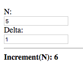
The value given to the delta (d) argument of increment is the initial value given for Delta, which is 1.

Now try changing Delta:

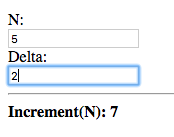
The value of the increment(n) node is updated, with the new value of Delta given as the delta argument. This shows that a binding is established rather than simply taking the value of the delta node.

4.4. Recursive Meta-Nodes

A recursive meta-node contains an instance of itself in its definition.

The following are the classic examples of recursion:

Example: Factorial.

factorial(n) :
    case(
        n < 1 : 1,  # Ignoring the case: n < 0
        n * factorial(n - 1)
    )

Example: Fibonacci Numbers.

fib(n) :
    case(
        n <= 1 : 1,
        fib(n - 1) + fib(n - 2)
    )

Recursion is the means by which Tridash provides iteration. The definition of factorial, above, will result in the stack space being exhausted for large values of n. This is due to the fact that each invocation of the meta-node consumes a certain amount of stack space. Since the recursive call to factorial has to be evaluated before the return value of the current call can be computed, the meta-node consumes an amount of stack space proportional to the value of n.

If the definition is rewritten such that it is tail recursive, that is the return value of factorial is the return value of the recursive call, a constant amount of stack space is consumed.

Example: Tail-Recursive Factorial.

factorial(n, acc : 1) :
    case(
        n < 1 : acc,  # Ignoring the case: n < 0
        factorial(n - 1, n * acc)
    )

This definition of factorial is tail recursive since the recursive call appears directly as the default value of the case expression, which is simply returned without any further operations performed on it.

In the previous implementation, the multiplication was performed on the result of the recursive call to factorial. In this implementation, the multiplication is performed on an accumulator argument, acc which is passed on to the recursive call and eventually returned when factorial is called with n < 1.


	Tridash supports general tail call optimization for mutually recursive meta-nodes.

4.5. Nested Meta-Nodes

A meta-node may contain other meta-nodes inside its definition. These meta-nodes may only be used within the body of the meta-node and shadow meta-nodes, declared in the enclosing scope, with the same identifiers.

With nested meta-nodes we can rewrite our previous tail-recursive factorial meta-node without having to expose the accumulator argument acc, which is an implementation detail.

Example: Factorial with nested iter meta-node.

factorial(n) : {
    iter(n, acc) : {
        case(
            n < 1 : acc,  # Ignoring the case: n < 0
            iter(n - 1, n * acc)
        )
    }

    iter(n, 1)
}

The computation of the factorial is implemented in the nested tail-recursive meta-node iter. The factorial meta-node simply calls this meta-node with the initial value for the accumulator.

4.6. Local Nodes

Nodes which appear as the target (observer) of a binding, declared within the body of a meta-node, are local to the meta-node’s body and may only be referenced within it. These may be used to store intermediate results or to break up complex expression into multiple nodes.

Example: Average.

average(a, b) : {
    sum <- a + b    
    sum / 2
}

Node sum is the binding target in this declaration.

In this example a local node sum is created, since it is bound (as the target) to the value of a + b. The value returned by average is the value of sum divided by 2.

4.7. Referencing Outer Nodes

A meta-node may reference nodes declared in the global scope or the enclosing scope(s) containing the meta-node definition. This creates a binding between the referenced node and each instance of the meta-node. The net result is that whenever the value of the referenced node changes, the value of the instance is recomputed. In essence a reference to an outer node can be thought of as an additional hidden argument.


	An outer node with the same identifier as a local node can be referenced with the `..` operator, e.g. `..(x)`.

Outer node references can be demonstrated by changing the definition of increment, in the Increment Application developed earlier in this tutorial, to the following:

Increment with reference to delta.

increment(n) : n + delta

The d argument has been removed and replaced with delta in the body.

Repeat the same experiment, changing the delta. You should observe the same results.

4.8. Fun Example: Simple Meter

In this example we’ll be developing an application which displays a simple meter, representing a quantity, which changes color as the quantity approaches the maximum.

Let’s start off with the following HTML interface:

ui.html.

<!doctype html>
<html>
    <head>
      <title>Simple Meter</title>
      <style>
        .meter-box {
            margin-top: 5px;
            width: 200px;
            height: 1em;
            border: 1px solid black;
        }
        .meter-bar {
            height: 100%;
        }
      </style>
    </head>
    <body>
      <h1>Simple Meter</h1>
      <div><label>Maximum: <input value="<?@ to-real(maximum) ?>"/></label></div>
      <div><label>Quantity: <input value="<?@ to-real(quantity) ?>"/></label></div>
      <div class="meter-box">
        <div id="meter" class="meter-bar"></div>
      </div>
    </body>
</html>


	The file contains a few CSS class definitions for styling the elements which display the meter, located at the bottom of the file.


	The `to-real` meta-node is similar to `to-int` except that it converts its argument to a real number rather than an integer.

The interface consists of two input fields for entering the values for the Maximum and Quantity, which are bound to the nodes maximum and quantity, respectively.

We’d like the meter to be displayed in a color which is in between green (empty) and red (full) depending on where the value of the quantity lies between 0 and the maximum.

First we’ll write a utility meta-node lerp for linearly interpolating between two values:

Meta-Node lerp.

lerp(a, b, alpha) : a + alpha * (b - a)

The value returned by lerp is the value between a and b proportional to where alpha lies between 0 and 1.

This meta-node will be used to interpolate between green and red depending on where the quantity lies between 0 and the maximum.

We can compute the value for alpha by dividing the value for the quantity by the maximum.

scale <- quantity / maximum


	This assumes that `maximum` is not 0.

Before we perform the interpolation, we need to make sure that scale is a value between 0 and 1. Let’s write another utility meta-node clamp which clamps a value to a given range.

Meta-Node clamp.

clamp(x, min, max) :
    case (
        x < min : min,
        x > max : max,
        x
    )

This meta-node returns the value of its first argument x if it is between min and max, otherwise returns min if x is less than min, or max if x is greater than max.

We can amend the computation of scale such that it does not exceed 0 and 1, by using the clamp meta-node.

scale <- clamp(quantity / maximum, 0, 1)

Finally we can interpolate between the two colours. We’ll be using the HSL (Hue Saturation Luminance) colorspace, and interpolating in the Hue component.


	The HSL, rather than the RGB, colorspace was used as it provides better interpolation results.

hue <- lerp(120, 0, scale)

hue is bound to a value interpolated between green (Hue 120) and red (Hue 0) with the value of scale as the interpolation coefficient.

Before we bind the interpolated color to the color of the meter, let’s write another utility meta-node which takes values for the hue, saturation and luminance components and produces a CSS HSL color string.

Meta-Node make-hsl.

make-hsl(h, s, l) :
    format("hsl(%s,%s%%,%s%%)", h, s, l)

The format meta-node produces a string in which %s placeholders in the format string (the first argument) are replaced with the values of the corresponding arguments (following the format string). %% placeholders are replaced with literal % characters.

format("Hello %s %s.", "John", "Smith") produces the string “Hello John Smith.”, as the first %s is replaced with "John" and the second %s is replaced with "Smith".

We can now generate a valid CSS color string using make-hsl that we’ll bind to the color of the meter element, which is the element with ID meter.

self.meter.style.backgroundColor <-
    make-hsl(hue, 90, 45)


	The `backgroundColor` style attribute references the background color of an element.

The constant values 90 and 45 have been chosen for the saturation and luminance components.

The last thing we need to do is adjust the width of the meter depending on the quantity value. We’ll simply multiply the value of scale by 100, to convert it to a percentage (indicating it should occupy that percentage of the width of its parent element), and bind it to the meter element’s width attribute.

format("%s%%", scale * 100) -> self.meter.style.width

Our application is complete. Add the following Tridash code tag to the top of the ui.html file.

<?
 /import(core)

 # Utilities

 lerp(a, b, alpha) : a + alpha * (b - a)

 clamp(x, min, max) :
     case (
         x < min : min,
         x > max : max,
         x
     )

 make-hsl(h, s, l) :
     format("hsl(%s,%s%%,%s%%)", h, s, l)


 # Application Logic

 scale <- clamp(quantity / maximum, 0, 1)

 hue <- lerp(120, 0, scale)

 self.meter.style.backgroundColor <-
     make-hsl(hue, 90, 45)

 format("%s%%", scale * 100) -> self.meter.style.width
?>

Build and run the application, and enter some values for the quantity and maximum, such that the quantity is less than half the maximum.

Maximum: 100, Quantity: 20, [Almost empty bright green meter]

Maximum: 100, Quantity: 40, [Almost empty dull green meter]

The meter is mostly empty and displayed in a green color.

Now increase the quantity such that it is greater than half the maximum.

Maximum: 100, Quantity: 60, [Half full yellow meter]

Maximum: 100, Quantity: 90, [Almost full red meter]

The meter is more than half full and its color approaches red as the quantity approaches the maximum.